Innovative Ptree Technology for Efficient Data Mining and Scalability
Our approach leverages vertical, compressed data structures known as Predicate-trees (Ptrees) to enhance scalability and address the challenges of dimensionality in data mining. Unlike conventional horizontal data processing methods, our Ptrees are designed to project attributes vertically, allowing for optimized data structures that can handle large datasets more efficiently. This patent-pending technology, developed by North Dakota State University, transforms how we structure and query data, focusing on purity and effective compression for better performance in data-driven applications.

Innovative Ptree Technology for Efficient Data Mining and Scalability
E N D
Presentation Transcript
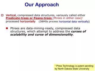
Our Approach • Vertical, compressed data structures, variously called either Predicate-trees or Peano-trees (Ptrees in either case)1 processed horizontally(DBMSs processhorizontal data vertically) • Ptrees are data-mining-ready, compressed data structures, which attempt to address the curses of scalability and curse of dimensionality. 1 Ptree Technology is patent pending by North Dakota State University
Predicate tree technology: vertically project each attribute, Current practice: Structure data into horizontal records. R( A1 A2 A3 A4) R[A1] R[A2] R[A3] R[A4] 010 111 110 001 011 111 110 000 010 110 101 001 010 111 101 111 101 010 001 100 010 010 001 101 111 000 001 100 111 000 001 100 010 111 110 001 011 111 110 000 010 110 101 001 010 111 101 111 101 010 001 100 010 010 001 101 111 000 001 100 111 000 001 100 Horizontally structured records Scanned vertically pure1? true=1 pure1? false=0 R11 R12 R13 R21 R22 R23 R31 R32 R33 R41 R42 R43 0 1 0 1 1 1 1 1 0 0 0 1 0 1 1 1 1 1 1 1 0 0 0 0 0 1 0 1 1 0 1 0 1 0 0 1 0 1 0 1 1 1 1 0 1 1 1 1 1 0 1 0 1 0 0 0 1 1 0 0 0 1 0 0 1 0 0 0 1 1 0 1 1 1 1 0 0 0 0 0 1 1 0 0 1 1 1 0 0 0 0 0 1 1 0 0 pure1? false=0 pure1? false=0 pure1? false=0 0 0 0 1 0 01 0 1 0 1 0 0 1 0 0 1 01 1. Whole is pure1? false 0 P11 P12 P13 P21 P22 P23 P31 P32 P33 P41 P42 P43 2. Left half pure1? false 0 P11 0 0 0 0 1 01 3. Right half pure1? false 0 0 0 0 0 1 0 0 10 01 0 0 0 1 0 0 0 0 0 0 0 1 01 10 0 0 0 0 1 10 0 0 0 0 1 10 0 0 0 0 0 0 0 0 0 0 0 0 0 1 1 0 0 0 0 1 10 0 0 0 0 1 0 1 0 0 ^ ^ ^ ^ ^ ^ ^ ^ ^ 0 0 1 0 1 4. Left half of rt half? false0 ^ 7 0 1 4 0 0 1 0 1 01 5. Rt half of right half? true1 0 1 0 6. Lf half of lf of rt? true1 To count occurrences of 7,0,1,4 use pure111000001100: 0 23-level P11^P12^P13^P’21^P’22^P’23^P’31^P’32^P33^P41^P’42^P’43 = 0 0 22-level=2 01 21-level ^ 7. Rt half of lf of rt? false0 then vertically project each bit position of each attribute, then compress each bit slice into a basic Ptree. e.g., compression of R11 into P11 goes as follows: Process vertically (vertical scans) R11 0 0 0 0 1 0 1 1 The compressed Ptree (1-Dim) version of R11, denoted, P11, is built by recording the truth of the predicate “pure 1” in a tree recursively on halves, until purity is achieved. Horizontally AND basic Ptrees P11 And it’s pure so branch ends But it is pure (pure0) so this branch ends
R11 R11 0 0 0 0 1 0 1 1 0 0 0 0 1 0 1 1 RL110:000 1:100 0:101 1:110 RL110:000 1:100 0:101 1:110 1. Whole file is true 1 1. Whole file is not pure1 0 2. 1st half is false 0 2. 1st half is not pure1 0 3. 2nd half is not pure1 0 3. 2nd half is true 1 0 0 0 0 1 1 0 0 0 0 0 0 0 0 1 0 0 0 0 0 1 0 1 1 1 10 1 0 1 1 1 0 1 1 0 1 1 1 1 0 1 0 1 1 1 1 0 0 0 0 1 10 0 1 4. 1st half of 2nd half not 0 4. 1st half of 2nd half true 1 5. 2nd half of 2nd half is 1 5. 2nd half of 2nd half true 1 6. 1st half of 1st of 2nd true 1 6. 1st half of 1st of 2nd is 1 7. 2nd half of 1st of 2nd not 0 7. 2nd of 1st of 2nd false 0 RunListTrees? (RLtrees) To facilitate subsetting (isolating a subset) and processing, a Ptree stucture can be constructed as follows: Or, a separate NotPure0 index tree (trees could be terminated at any level). 1st, AND NP0trees. Only 1-branches / result need ANDing thru list scans. The more operands, the fewer 1-branches.
start length P0RI11000:4101:1 R11 pattern 0 0 0 0 1 0 1 1 0 1 0 1 0 1 0 1 Length (# of consecutive replicas of pattern) RL110:01:1000:101 1:11001:1000 P1RI11100:1110:2 PLZVRI111000:1 Other Indexes on RunLists We could put Pure0-Run, Pure1-Run and even Mixed-Run (or LZV-Run) RunListIndexes on RL:
Best Pure1 tree Implementation? My guess circa 04jan For n-D Pure1 trees: • At any node, if |1-bits| in the tuple set represented by the node < lower threshold, LT, • Then that node will simply show the 1List, the list of 1-bit positions (use a 0-bit if =0) and have no children, • Else if the tuple set represented by that node < UT=2nm, anupper threshold, leave bit-slice uncompressed Building such Ptrees bottom up: Using in-order ordering, • If 1-count of the next UT-segment LT install P-sequence, else install 1List. • If current UT-segment node is numbered k*(2n–1) and it and all 2n-1 predecessors are 1Lists, and the cardinality of the union of said 1Lists < LT, install the union in the parent node. Recurse this collapsing process upward to the root. Building such Ptrees top down: • For datasets larger than UT, recursively build down the pure1. • If ever a node has < LT 1-bits, install the 1List and terminate that branch. • At the level where the represented tuple set = UT, install 1List if |1-bits| < LT, else install P-sequence. Notes: • This method should extend well to data streams. When the data stream exceeds the current allocation (which, for n-D Ptrees will be a power of 2n), just grow the root of each Ptree to a new level, using the current Ptree as node 0. Nodes 1,2,3,…2n-1 of the new Ptree will start as 0 nodes without children and will grow as 1Lists until LLT is reach then they will be converted to P-sequences.
Vertical, compressed, lossless structures that facilitates fast horizontal AND-processing P-trees are all of the following: Partition-tree: Tree of nested partitions: Root is the entire bit sequence Level-1 is a partition of the root P(R)={C1..Cn} In level-2 each level-1 component is partitioned by P(Ci ) = {Ci,1..Ci,ni} i=1..n, In level-3 each level-2 component is partitioned by P(Ci,j) = {Ci,j1..Ci,jnij} ... Ptrees Partition tree R / … \ C1 … Cn /…\ … /…\ C11…C1,n1Cn1…Cn,nn . . . Predicate-tree: For a predicate on the leaf-nodes of a partition-tree (also induces predicates on i-nodes using quantifiers) Predicate-tree nodes can be truth-values (Boolean P-tree) Predicate can be quantified existentially (1 or a threshold %) or universally Purity-tree: universally quantified tree (predicate is “1 position) , Pure1-tree) existential quantified tree (predicate is “ a 1 position), NotPure0-tree) We will focus on P1trees. All Ptrees shown so far were 1-dimensional (recursively partition by halving bit files),but they can be 2-D (recursively quartering) (e.g., used for 2-D images) 3-D (recursively eighth-ing), … Or based on purity runs or LZW-runs or …
Best Ptree Implementation? My guess circa 04feb Ptrees can be viewed “breadth first bottom up ” That is, one can view the leaf level (level-0) horizontally and then view level-1 as another bit vector in which each bit represents the truth of the predicate (e.g., pure1), applied to pairs of bits in the leaf level vector. This can be continued upwards for each successive level until the root is reached. The result is a bottom up construction of the 1-D ptree. This construction has the advantages that the leaf level vector can be any length and can grow (e.g., for data streams) , Each level up e.g., level-k, can be grown as new 2k-granules for that level fill up. Additionally, the breadth-first bottom up view of the 2-D ptree for that bit vector is just the leaf vector with every other level above it left out. The breadth first bottom up view of the 3-D ptree is just the leaf level then leaving out 2 consecutive levels at a time, going up the levels. 4-D is the same leaving out triples of levels at a time, etc. Another advantage of this view is that, stripping an additional k levels just above the leaf level amounts to using 2k length p-sequence at the leaf as discussed discussed on a previous slide. The breadth-first bottom up (B2U) view doubles the storage requirement over the storage requirement of p-sequences. However, storage is free so it isn’t a big concern. The capture time (on the DII side) is probably much higher, but that is a one-time cost. On the face of it, compression is gone. However, we are talking about disk space again, which is free. In terms of anding speed, the compression is there (just don’t decent on purity). However, one should have the NZ trees (for the existential case) as well in order to distinguish purity. Note, we are replacing all pointers with offsets now, so distinguishing mixed from pure zero cannot be done by “no child pointers”.