Carbon Dioxide Simulator
Carbon Dioxide Simulator. Data from: http://www.esrl.noaa.gov/gmd/ccgg/trends/. Carbon Dioxide Simulator. www.atmosedu.com/meteor/ejs/ejs_CO2C.jar.

Carbon Dioxide Simulator
E N D
Presentation Transcript
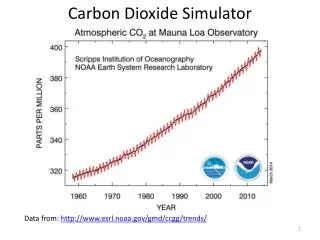
Carbon Dioxide Simulator Data from: http://www.esrl.noaa.gov/gmd/ccgg/trends/
Carbon Dioxide Simulator www.atmosedu.com/meteor/ejs/ejs_CO2C.jar Simulator environment is a stand alone JAVA program. Download it and open it up to run. Two window will be available. 1. description 2. the simulator. The link below is to the downloadable Java Carbon simulator To model details
Mauna Loa annual mean CO2 values for model comparison MS Excel document with graph and data www.atmosedu.com/meteor/ejs/CarbonBudget.xls
Fossil Fuel and Cement emissions from 1960 to 2012 are fixed in simulator at NOAA estimates http://cdiac.ornl.gov/GCP/carbonbudget/2013/ (source of above estimates)
1960 to 2012 Carbon emissions from Land Cover Change (LCC) are fixed in simulator at estimates provided by R. Houghton Personal communication (2013) MS Excel document with graph and data www.atmosedu.com/meteor/ejs/CarbonBudget.xls
Carbon Dioxide Simulator (default window) Graphical Output Note that the x-axis labels here are 1960 to 2010 Numeric Output table (scrollable) Slider to adjust Terrestrial carbon Sink Click to see default emission scenario Run Reset Buttons
Slider to adjust Terrestrial carbon Sink Pan et al (2011) estimate that the net Global terrestrial carbon sink is 1.1 +/- 0.8 GtC/yrand is mostly located in temperate and boreal forest regions. A Large and Persistent Carbon Sink in the World's Forests Science 333, 988 (2011); YudePan et al.
Note on input The assume value of the terrestrial carbon sink can be controlled by the slider or typing directly into the text box. All textbox entries this simulator must be finalized by pressing the Enter (Return) key your the computer. The yellow highlight above warns that the entry has not yet been made.
Note on output + Hold the cursor down X=2010 y=389 Values appear in output box
Note on output Scrollable data table Second column is model simulated atmospheric Carbon dioxide (ppt) Last column is the net atmospheric carbon source –sink (in GtC/yr) =(Fossil Fuel and Cement Emissions)+( Emissions from Land Cover Change)-(Terrestrial Sink)
First task: • Adjust the Terrestrial sink to achieve your best fit between model simulation and Mauna Loa CO2 observations. • Using Pan et al. estimates of 1.1+/- 0.8 (GtC/yr) for the terrestrial sink run three simulations: Terrestrial sink =0.3, 1.1, and 1.9 (GtC/yr) • Graph all three simulations on the same axes and discuss your results (200 word minimum). • In your discussion include: • The range of 2010 CO2 v
Future Carbon Dioxide Projections Both x and y axes change x-2000 to 2100 y 350 to 1350 (ppm) Input for future emission Scenarios become available 2. Select radio button for 200 to 2100 run 1. reset
The Business as usual scenario (A1F1) can be approximated by 4 percent growth time intervals. The simulation environment allows the user to change these 4 growth rates. This is the default simulation for future projections.
Global Fossil Fuel and Cement Carbon Emission (FFE) estimates (GtC/yr) http://cdiac.ornl.gov/GCP/carbonbudget/2013/(FFE estimates) 2000 to 2015 assumed growth of 3% fits emission estimates. This is slightly higher than the business as usual scenario.
Four examples of user controlled future fossil fuel emission scenarios
Example future scenario RunsBAU and zero emission growth after 2012 CO2 graph This graph is available from clicking on emissions graph
Task 2 • Find an emission scenario that keeps CO2 levels from going above 450 ppm. Paste both the CO2 graph and the emission graph into your report for this scenario. Comment on the feasibility of this scenario (100 words minimum)
Task 3 • Reset & check 2000 to 2100 run • Run Default simulation (BAU) • Run a simulation with 2013 to 2030 growth rate =-100%. This is very unrealistic. • Paste both the CO2 graph and the emission graph into your report for this scenario. Comment on the results of this scenario (100 words minimum). The idea here is that all emissions are suddenly (and magically) cut to zero but the year 2100 CO2 concentration seems to stay above preindustrial level of 280. Why is this true? How long do you think it will take for the emissions to get back to preindustrial levels?
Task 4________ • Run the three runs shown in the table above and record the year 2030 and year 2060 CO2 values for each simulation. Also record the BAU-half and half – zero differences.
Task 4 (cont) • How do the 2030 concentrations for the three different scenarios of Table 2 compare with each other? • How do the 2060 concentrations for the three different scenarios of Table 2 compare with each other?
T/F the predicted 2030 concentration depends very strongly on the assumed emission scenario. T/F the predicted 2060 concentration depends very strongly on the assumed emission scenario. A policy change aimed at limiting carbon dioxide in the atmosphere that is implemented by a political agreement today will take ____________ years to result in observable differences in the amount of carbon dioxide in the atmosphere. • 5 years • 10 years • 20 years • More than 20 years
Based on your answers above and any other potentially important factors, discuss the political incentives and disincentives to proposing legislation to curtail carbon emissions. (100 words)
Task 5 Devise your best future emission scenario for estimating atmospheric carbon dioxide concentrations for the rest of this century. Use a web based search and your intuition for rationale in selecting your emission scenario. (explain your rationale 100 words minimum)
Task 5 continued • Paste both the CO2 graph and the emission graph into your report for this scenario. • Use the assumption that limiting atmospheric CO2 concentration to 450 ppm or below will result in adaptable climate change as a benchmark to discuss to possible implication of your emission scenario to our future climate. (100 words minimum)
Carbon Dioxide Java Simulator Modelbrief overview By R.M. MacKay
The simulator is designed to capture the global carbon cycle’s influence of the future behavior of atmospheric carbon dioxide after some emission into the atmosphere.
The formulation in the above paper is used by us to estimate the future response of atmospheric carbon dioxide to anthropogenic forcing. It is also the basis of global warming potential calculations used by working group 1 of the IPCC (2013).
Schematic implementation of the impulse response function of Joos et al. 2013 When carbon is injected into the atmosphere in a given year, 27.6 % goes into a rapid response component of the carbon cycle (4.30 yr decay time), 28.2 % goes into a moderate response component (36.5 yr decay time), 22.4 % goes into a long term response component (394 yr decay time), and 21.7 % never leaves. This captures the mean response of more sophisticated carbon cycle models for time scales less than 1000 yrs. The carbon cycle component with the shortest lifetime accumulates the least carbon over time.