Light Interference and Localization in Strongly Driven Multi-Particle Systems
370 likes | 516 Vues
This study investigates the spatial distribution of spontaneous emission and interference patterns in multi-particle systems. It explores weak and strong-field spatial interference, highlighting two-photon spatial coherences in atoms under strong drives. The work utilizes Cauchy-Schwarz inequalities and examines localization of atomic ensembles via super-radiance. Key questions include enhancing spatial resolution and returning to first-order interference under strong laser fields. Techniques studied could lead to accurate sub-wavelength localization of atomic ensembles, contributing to fields such as quantum optics and condensed matter physics.

Light Interference and Localization in Strongly Driven Multi-Particle Systems
E N D
Presentation Transcript
Light interference and localization of strongly driven multi-particle systems Mihai Macovei, JÖrg Evers and Christoph H. Keitel Max-Planck Institute for Nuclear Physics, Heidelberg, Germany CEWQO 2007, Palermo, Italy
Outline • Motivation • Spatial distribution of spontaneous emission • Weak and strong-field spatial interference • Two – photon spatial coherences in strongly driven regular multi-particle structures. • Cauchy-Schwarz inequalities • Localization of atomic ensembles via super-fluorescence • Conclusions
Motivation Fundamental questions • recovering the first-order spatial interference for stronger laser fields, • improving the spatial light-resolution, • investigating the spatial behaviors of quantum properties of light • to localize atomic ensembles with a sub-wavelength accuracy • multi-particle systems, • single- and two-photon interference, • sub-wavelength localization.
Spatial distribution of spontaneous emission • The spontaneous emission of non-interacting excited particles in vacuum is isotropic. • The collective spontaneous emission of an excited pencil-shaped two-state system is distributed along the sample’s axis. M. Gross and S. Haroche, Phys. Rep. 93(5), 301 (1982).
Spatial interference Double slit with two trapped ions: applications e.g. in lithography? U. Eichmann et al., Phys. Rev. Lett. 70, 2359 (1993)
Two-atom collective states Introduce new state basis: dark-center interference bright-center interference Two transition amplitudes add with different phases: - + bright center dark center via symmetric state via anti-symmetric state C. Skornia et al., Phys. Rev. A 64, 063801 (2001)
Analytical methods. Approximations • Master equation approach • Dipole and rotating - wave approximations • Mean-field and Born - Markov approximations • Dressed - states formalism • Secular approximation.
Weak- field spatial interference. Visibility For weak fields, the visibility of the interference pattern is if Note that V0 when >> γ.
bare states dressed states The strong field case Spectral decomposition: under strong driving: splitting in different spectral bands Mollow spectrum define observables for each spectral band separately
Recovering strong-field interference Ansatz: modify mode density at dressed-state transition frequencies e.g. via cavity this changes spontaneous emission and redistributes populations look at single spectral band change mode density via cavity “right” sideband suppressed “left” sideband suppressed
Strong - field spatial interference. Spectral -line intensities
Strong-field spatial interference in a tailored electromagnetic bath One can define separately the visibilities V = (Imax-Imin)/(Imax+ Imin) for each of the central, left and right spectral lines, respectively. Central band visibility VCB as a function of = γ(ω+)/γ(ω-). no interference in plain vacuum, η = 1
Strong-field spatial interference. Regular atomic structures
The strong-field spatial interference pattern ... ... Central-band intensity ICB/N2 as function of α1. Here kLrab=20π and VCB= 0.9. Blue line: N=8, red curve: N=2. M. Macovei, J. Evers, G.-x. Li, C. H. Keitel, Phys. Rev. Lett. 98, 043602 (2007).
Two-photon spatial coherences in strongly driven multi-particle structures
Two-photon spatial coherences The coherence properties of an electromagnetic field, at space-point R, can be evaluated with the help of the second-order coherence functions: where are the creation (annihilation) operator for modes { i, j }. can be interpreted as a measure for the probability for detecting one photon emitted in mode i and another photon emitted in mode j with delay τ. The quantity
Second-order correlation functions. Properties Equal times: g2( τ = 0 ) = 1 : poissonian photon statistics (e.g. coherent state) g2( τ = 0 ) < 1 : sub-poissonian photon statistics (e.g. Fock state) g2( τ = 0 ) > 1 : super-poissonian photon statistics (e.g. thermal light) Different times: g2( τ > 0 ) ≤ g2( τ = 0 ) : bunching (e.g. thermal light) g2( τ > 0 ) > g2( τ = 0 ) : anti-bunching (e.g. single atom fluorescence) Non-classical: g2( τ > 0 ) > g2( τ = 0 ) g2( τ = 0 ) < 1
Cauchy-Schwarz inequalities The Cauchy-Schwarz inequalities are violated if i.e., if the cross-correlation between photons emitted into two different modes are larger than the correlation between photons emitted into individual modes.
Second-order spatial interference resolution The central-band second-order correlation function. The red line depicts the strong-field limit (Vc=0) while the blue curve describes the weak-field case with N=2, and M. Macovei, J. Evers, G.-x. Li, C. H. Keitel, Phys. Rev. Lett. 98, 043602 (2007).
Summary • The strong-field first order interference pattern can be recovered by tailoring the electromagnetic reservoir surrounding the atomic structure • Second order correlation functions do exhibit interference effects even in the standard vacuum. • The cross-correlations between photons emitted in the spectral sidebands violate Cauchy-Schwartz inequalities and their emission ordering cannot be predicted.
Localization of atomic ensembles via super-fluorescence M. Macovei, J. Evers, C. H. Keitel, M. S. Zubairy, Phys. Rev. A 75, 033801 (2007)
Multi-particle sub-wavelength localisation. Approach sample of atoms Localization of ensembles atoms are positioned in a standing wave laser field sample has linear dimensions smaller than wavelength atoms dipole-dipole interact Dicke model collective operators, e.g.
The Hamiltonian Free energies Atom-lasercoupling Atom-vacuum coupling
Master equation: - ] Coherent part Spontaneous emission Dipole-dipole coupling
Steady-state solution Ansatz for steady state: Bosonic ladder operators Inserting in Master equation yields analytic solution:
Steady-state solution Ansatz for steady state: Bosonic ladder operators Inserting in Master equation yields analytic solution:
Fluorescence intensity profile Ω / (Nγ) = 100 Ω / (Nγ) = 50 Ω / (Nγ) = 25 Ωd = -10 γ Δ/(Nγ) = 0.5 width ~ 0.01 λ node Intensity dip width can becontrolled Intensity Position in standing wave
node Intensity Position in standing wave Fluorescence intensity profile 2 atoms 4 atoms 8 atoms Ω = 100 γ Ωd = -5 γ Δ = 10 γ
Interpretation Two atom case: For small distances, anti-symmetricstate decouples Minimum dip width aroundposition of symmetric state detuning position Many atom case: Minimum width around positionwhere symmetric states are No structure at positions ofantisymmetric states But positions not exactlydefined because of many(anti-) symmetric states detuning position
Scanning-dip spectroscopy Change phase of standingwave field to move nodes Constantly monitorscattered light intensity Identify position of atomsvia the absence of lightat the nodes→ localized particles unperturbed accuracy determined bydip width Intensity dip should be as narrow as possible
Single-pass localization Collection flying through cavity: Only short interaction Try to obtain as much information as possible Measurement scheme: The total amount of scatteredlight provides localization information Measured intensity fixeshorizontal cut and thusposition range Large slope of intensity profile desirable over whole wavelength
Summary Localization of atomic ensembles ensemble confined to region smaller than wavelength evaluate fluorescence in standing wave field→ collective effects Scanning-dip localization relies on the absence of fluorescence→ localized particle essentially unperturbed exploits collectivity and strongfields to tailor a narrow dipin fluorescence profile Single-pass localization gain as much position informationas possible in single pass requires a wide dip in fluorescence profile in order to work at all positions