Download
1 / 34
380 likes | 559 Vues
The control surface A can be considered to consist of three regions: A in : the surface of the the region where the fluid enters the control volume; A out : the surface of the region where the fluid leaves A wall ; the fluid is in contact with a wall. A = A in + A out + A wall.

E N D
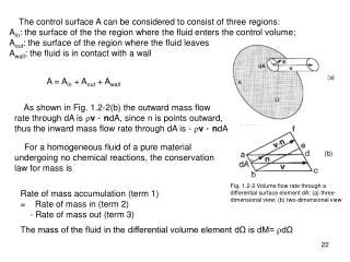
The control surface A can be considered to consist of three regions: Ain: the surface of the the region where the fluid enters the control volume; Aout: the surface of the region where the fluid leaves Awall; the fluid is in contact with a wall A = Ain + Aout + Awall As shown in Fig. 1.2-2(b) the outward mass flow rate through dA is rv.ndA, since n is points outward, thus the inward mass flow rate through dA is - rv.ndA For a homogeneous fluid of a pure material undergoing no chemical reactions, the conservation law for mass is (b) Fig. 1.2-2 Volume flow rate through a differential surface element dA: (a) three- dimensional view; (b) two-dimensional view Rate of mass accumulation (term 1) = Rate of mass in (term 2) - Rate of mass out (term 3) The mass of the fluid in the differential volume element dΩ is dM= rdΩ
The mass of the fluid in the differential volume element dΩ is dM= rdΩ The total mass in the control volume is M = The rate of mass change in the control volume is The net inward mass flow rate into Ω is That is [1.2-4] Examples 1.2-1 and 1.2-2
1.3 Differential mass-balance equation According to Eq. 1.2-4 [1.2-4] [1.3-1’] According to Gauss divergence theorem [A.4-1] [1.3-2] Substituting Eq.[1.3-1’] and [1.3-2] into [1.2-4], we obtained [1.3-3] The integrand must be zero everywhere since the equation must hold for any arbitrary Ω. Therefore, we have [1.3-4]
Equation [1.4-4] is the differential mass-balance equation, that is, the equation of continuity. For an incompressible fluid, the density r is constant and Eq. 1.3-4 becomes Example 1.3-2 Normal stress due to creeping flow around a sphere
Rate of momentum in Rate of momentum out Sum of forces acting on system Rate of momentum accumulation - = + 1.4 Overall momentum-balance equation Consider an arbitrary stationary control volume Ω bounded by surface A through a moving fluid is flowing, as shown in Fig. 1.4-1. The control surface A can be considered to consist of three parts: A = Ain + Aout + Awall Consider conservation law for momentum of the control volume: [1.4-2] This equation is consistent with Newton’s second law of motion The mass contained in a differential volume element dΩ in the control volume is rdΩ and its momentum is dP = rvdΩ. The momentum of the fluid in Ω is :
The rate of momentum change in Ω is : [1.4-a] The inward mass flow rate through dA : -r(v.n)dA The inward momentum flow rate through dA : -rv(v.n)dA The net inward momentum flow rate into Ω : or Since v = 0 at the wall, the equation can be expressed as Define v =|v.n| [1.4-b]
The pressure force acting on dA is dFp = -pndA, The pressure force acting on the entire control surface A is [1.4-c] The viscous force exerted on the fluid by the surrounding over dA is dFv = -t‧ndA, the viscous force exerted on the fluid by the surroundings over A is [1.4-d] The body force acting on the differential volume element dΩ is dFb = fbdΩ, the body force acting on the entire control volume is [1.4-e] Substituting [1.4-a] through [1.4-e] into [1.4-2] [1.4-3] or
[1.4-8] Where P = momentum of fluid in control volume m = mass flow rate at inlet or outlet Fp = pressure force acting on control volume by surrounding Fv = viscous force acting on control volume by surrounding Fb = body force acting on control volume The correction factor a a = 4/3 for laminar flow in round pipes ~ 1 for turbulent flow
1.5 Differential momentum-balance equation 1.5.1 Derivation Eq. 1.4-3 represented the integral form of momentum-balance equation [1.5-1] The surface integrals in Eq. 1.5-1 can be converted into their corresponding volume integrals. From Eq. [A.4-4], we have Eq. 1.5-1 can be rewritten as follows:
The integrand must be zero everywhere since the equation must hold for any arbitrary region Ω, therefore ∵ and It can be further simplified with the help of the equation of continuity as following: (for constant r and m) [1.5-8] If the gravity force is the only body force involved, that is [1.5-9] The equation is called Navier-Stokes equation
The equation of motion is often expressed in terms of the Stokes derivative D/Dt, Which is defined as follows: The equation of motion (Eq. 1.5-9) becomes (1) (2) (3) (4) Where term (1): the inertia force per unit volume, namely, the mass per unit volume times acceleration (2):pressure force, (3) viscous force, and (4) gravity force per unit volume
inertia force: pressure force: viscous force: gravity force: rg 1.5.2 Dimensionless form The equation of motion and the continuity equation can be expressed in the dimensionless form. In forced convection, a characteristic velocity V, length L, and time L/V are used to express the equation qualitatively. By substituting V for v, (L/V)-1 for D/Dt, L-1 for ▽, and L-2 for ▽2. Define: dimensionless velocity dimensionless pressure dimensionless time dimensionless coordinates Dimensionless operator Dimensionless operator
Substituting Eqs. [1.5-12] through [1.5-17] into Eqs.[1.5-18] and [1.5-19], we have Continuity: Motion: Multiplying Eq.[1.5-21] by L/V and Eq.[1.5-22] by L/rV2, we have Continuity: Motion:
Therefore, for forced convection Continuity: Motion: Where
Given a physical problem in which the dependent parameter is a function of n-1 independent parameters. We may express the relationship among the variables in functional form as where q1 is the dependent parameter, and q2, …, qn are n-1 independent parameters. Mathematically we can express the functional relationship in the equivalent form Where g is an unspecified function, different from f. The Buckingham Pi theorem states that: Given a relation among n parameters of the form then the n parameters may be grouped into n-m independent dimensionless ratios, or n parameters, expressed in a functional form by or The number m is usually, but not always, equal to the minimum number of independent dimensions required to specify the dimensions of all the parameters q1, q2, …and qn.
Example The drag force F, on a sphere depends on the relative velocity, V, the sphere diameter, D, the fluid density, r, and the fluid viscosity, m, Obtain a set of dimensionless groups that can be used to correlate experimental data. Given: F=f(r, V, D, m) for a smooth sphere Find: An appropriate set of dimensionless groups Solution: Step 1: Find the parameters: F, r, V, D, and m. n=5 Step 2: Select primary dimensions: M, L, t or F, L, t r=3 Step 3: Find the dimension of the parameters selected in step 1 F r V D m ML/t2 M/L3 L/t M/L3 M/(Lt) Step 4: Select repeating parameters with the number equal to the primary dimensions r, V, D m=3 Step 5: n-m=2. Two dimensionless groups will result. Step 6: Setting up dimensional equations Π1= raVbDcF, and Π2= rdVeDfm Step 7: Summing exponents
M: a+1 =0 => a = -1 L: -3a+b+c+1=0 => c = -2 Therefore T:-b-2=0 => b =-2 Similarly Step 8: Check using F, L, t dimensions and The functional relationship is Π1=f(Π2), or As noted before. The form of the function, f, must be determined experimentally.
Example 1.5-1 Tangential annual flow (Incompressible, Newtonian, laminar) Flow is in q direction only, vr=vz=gq=0 Flow is axisymmetric, no pressure variation in the q direction. Neglect end effects, The equation of continuity in cylinder coordinates is Which can be reduced to The velocity distribution vq(r), the q component of the equation of motion is The boundary conditions are vq =0 at r = r1, vq = r2w2 at r = r2
Example 1.5-2 Laminar flow through a vertical tube, find the velocity, volume flow rate, and shear stress (Steady-state, incompressible, Newtonian) Flow is in z direction only, vr=vq=0, vz is independent of q Subjected to B.Cs Find vav
Example 1.5-3 Flow of a rising film Continuity Eq. Eq. of motion B.Cs