LINEAR PROGRAMMING
LINEAR PROGRAMMING. 1.224J/ESD.204J TRANSPORTATION OPERATIONS, PLANNING AND CONTROL: CARRIER SYSTEMS Professor Cynthia Barnhart Professor Nigel H.M. Wilson Fall 2003. Announcements. Reader Problem set #1 December 1 recitation & December 5 class OPL Studio examples.

LINEAR PROGRAMMING
E N D
Presentation Transcript
LINEAR PROGRAMMING 1.224J/ESD.204J TRANSPORTATION OPERATIONS, PLANNING AND CONTROL: CARRIER SYSTEMS Professor Cynthia Barnhart Professor Nigel H.M. Wilson Fall 2003
Announcements • Reader • Problem set #1 • December 1 recitation & December 5 class • OPL Studio examples Barnhart 1.224J
LINEAR PROGRAMMING Sources: -Introduction to linear optimization (Bertsimas, Tsitsiklis) -Nathaniel Grier’s paper -1.224 previous material
Outline • Modeling problems as linear programs • Solving linear programs Barnhart 1.224J
Outline • Modeling problems as linear programs • What is a linear Program • Formulation • Set Notation Review • Example: Transit Ridership • Standard Form of an LP • Linearity • Examples Barnhart 1.224J
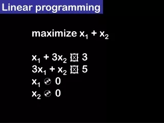
What is a Linear Program (LP)? • Objective Function • summarizes objective of the problem (MAX, MIN) • Constraints of problem: • limitations placed on the problem; control allowable solutions • Problem statement: ‘given….’, ‘must ensure…’, ‘subject to’ • Equations or inequalities • Decision Variables • quantities, decisions to be determined • multiple types (real numbers, non-negative, integer, binary) • In an LP, the decision variables are real numbers • Choice of decision variables will determine difficulty in formulating and solving the problem Barnhart 1.224J
Set Notation Review Set:collection of distinct objects R: set of real numbers Z: set of integers 0: emptyset Superscript +: non-negative elements of a set ∈ : ‘is an element of’ { } : ‘the set containing’ (members of the set are between brackets) : or | : ‘such that ’ example: {x ∈ S : x ≥ 0} ∃ :’there exists’ ∀ : ‘for all’ Barnhart 1.224J
Example: Transit Ridership • A transit agency is performing a review of the service it provides. It has decided to measure its overall effectiveness in terms of the total number of riders it serves. The agency operates a number of modes of transport. The table shows the average number of riders generated by each trip (by mode) and the cost of each trip (by mode) • Give a formulation of the problem to maximize the total number of riders the agency services given a fixed daily budget of $5,000. Barnhart 1.224J
Transit Ridership Formulation • Decision Variables? • X1= number of trips made using heavy rail • X2= number of trips made using light rail • X3= number of trips made using bus rapid transit (BRT) • X4= number of trips made using bus • Objective Function? • MAX (Total Ridership) • Ridership= 400*X1+125*X2+60*X3+40*X4 • Constraints? • Cost budget • Cost=200*X1+80*X2+40*X3+30*X4 Barnhart 1.224J
Transit Ridership Model Generalization: -M= set of modes -ri = average ridership per trip for mode i -ci= average cost per trip for mode i Barnhart 1.224J
Writing the model in OPL Studio Barnhart 1.224J
Transit Ridership: Additional Constraints Generalization • The agency wants to provide a minimum number of trips mi , for each mode i • The agency wants to provide service to a minimum number of riders bi , for each mode i . Generalization Barnhart 1.224J
Additional Constraints in OPL Studio Barnhart 1.224J
Standard Form of a LP Any LP can be reduced to its standard form: • Inequality constraints can be transformed into equality by adding « slack » variables • Max problem can be transformed into a MIN problem by reversing signs of objective function coefficients • Free variables can be eliminated by replacing them by xj+-xj , where xj+ and xj- are new variables such that xj+>=0 and xj->=0 => General problem can be transformed into standard form => only need to develop methods capable of solving standard form problems. Barnhart 1.224J
Linearity • In a LP, objective AND constraints MUST BE linear • MAX{x1,x2,…}, xi*yi, |xi|, etc => non-linear if xi and yi are variables • Sometimes there is a way to convert these types of constraints into linear constraints by adding some decison variables • Examples: Barnhart 1.224J
Dealing with absolute valuesExample Barnhart 1.224J
Dealing with minimizing piece-wise linear convex cost functions Example Cost such that: • What to do? • • Introduce a new variable T such that: • In linear form: Barnhart 1.224J
Example A marketing manager has an advertising budget of $150,000. In order to increase automobile sales, the firm is considering advertising in newspapers and on TV. The more a particular medium is used, the less effective is each additional ad. Each newspaper ad costs $1,000 and each TV ad costs $10,000. At most 30 newspaper ads and at most 15 TV ads can be placed. Barnhart 1.224J
Problem Formulation 1 x N1 : # of newspaper ads placed between 1-10 x N2 : # of newspaper ads placed between 11-20 x N3 : # of newspaper ads placed between 21-30 x T1 : # of TV ads placed between 1-5 x T2 : # of TV ads placed between 6-10 x T3 : # of TV ads placed between 11-15 What does this formulation rely on? Barnhart 1.224J
Alternative Formulation 2 Variables: X: number of customers reached via newspaper ads Y: number of customers reached via TV ads N: number of newspaper ads T: number of TV ads X and Y are piecewise linear functions of N and T respectively Maximize ( X + Y ) . . s.t Barnhart 1.224J
Alternative Formulation 3 xN: # of newspaper ads xT: # of TV ads placed yi: supplementary variables, i=1,2,…,6 Barnhart 1.224J
Additional ConstraintsHow would you model the following? (1) At most 30 ads can be placed in total (2) There is a 20% discount for each additional TV ad if the number of TV ads exceeds 12 (1) Add the following constraint: xN+ xT≤ 30 (2) Define a new supplementary variable ydand replace y6with y’6+ydin previous formulation, and add: Barnhart 1.224J
Formulating the Model • Multiple ways to develop a model formulation 1-Decide on an inital set of decision variables • Traditionally letters from the end of the alphabet, use of subscripts, ordering of subscripts 2-Determine objective function: – obtainable from problem statement • Can be very complex 3-Determine the constraints: • Variable-value constraints: non-negativity, binary constraints • Capacity constraints, demand constraints, balance flow constraints • Sometimes necessitates introduction of additional variables Barnhart 1.224J
Outline 2. Solving linear programs • Linear Programs: Forms and Notation • Basic/Non-basic variables • Dual Variables • Reduced Costs • Optimality Conditions • Example • Simplex algorithm • Sensitivity Analysis • Introduction of a new variable • Addition of a new constraint • Change in the cost coefficient of a non-basic variable • Change in the constraint coefficient of a non-basic variable Barnhart 1.224J
Linear programs: Form and notation • c in an n*1 vector • x is an n*1 vector • A is an m*n matrix • b is an m*1 vector Barnhart 1.224J
Basic Solutions • If an LP has an optimal solution, it must also have an optimal basic solution • A basic solution is one in which all but m variables take on value zero • n -m non-basic variables • These m variables are referred to as basic variables (note that basic variables can also take on value 0) Barnhart 1.224J
Dual Variables • Let π be the m*1 vector of dual variables associated with the m constraints • Given a basic solution, the dual variable value of a constraint can be interpreted as the value of relaxing the constraint by one unit. • If the constraint is not binding, the dual value is equal to 0 and relaxing it by one unit has no effect on the optimal solution Barnhart 1.224J
Reduced Costs The reduced cost of variable xiis: Reduced costs of a variable xican be viewed as an estimate of the change in the objective function value achieved by increasing xi by one unit. Barnhart 1.224J
Calculating reduced costs Barnhart 1.224J
Solving the LP • Many algorithms can be used to solve the LP • Simplex algorithm (most popular) • Searches for an optimal solution by moving from one basic solution to another, along the edges of the feasible polygon, in direction of cost decrease (Graphically, moves from corner to corner) • Interior Point Methods (more recent) • Approaches the situation through the interior of the convex polygon • Affine Scaling • Log Barrier Methods • Primal-dual methods Barnhart 1.224J
The Simplex algorithm for minimization problems 1-Compute the reduced costs of all non-basic variables. If they are all non-negative, stop. 2-If not, choose some non-basic variable with negative reduced cost. 3-Identify an active variable to remove from the basis. 4-Solve for the value of the new set of basic variables. 5-Solve for the new value of the dual variables. 6-Return to Step 1 Barnhart 1.224J
Simplex Optimality Conditions (for minimization problems) The current feasible solution x is optimal when: • The reduced costs of all basic variables equal 0 • Maintained at each iteration of the simplex algorithm • The reduced costs of all non-basic variables are non-negative • Not maintained at each iteration of the simplex algorithm • Dual variables are feasible for the dual problem • Complementary slackness is satisfied (maintained at each iteration of the simplex algorithm) • Dual variable value is zero unless its associated constraint is binding (has zero slack) • Value of the decision variable xiis zero unless its associated reduced cost is zero • xi is non-zero only if its associated reduced cost is zero. Barnhart 1.224J
Example* A company produces 3 products. Each unit of product 1,2, and 3 generate a profit of $10, $12 , and $12 respectively. Each product has to go through a manufacturing, assembly, and testing phase. The company’s resources are such that only 20 hours of manufacturing, 20 hours of assembly, and 20 hours of testing are available. Each unit of product 1 has to spend 1 hr in manufacturing, 2 hrs in assembly, and 2 hrs in testing. Each unit of product 2 has to spend 2 hrs in manufacturing, 1 hr in assembly, and 2 hrs in testing. Each unit of product 3 has to spend 2 hrs in manufacturing, 2 hrs in assembly, and 1 hr in testing. Company ABC wants to know how many units of each product it should produce, in order to maximize its profit. In Standard Form *Source: Optimization Methods p101 Barnhart 1.224J
In OPL Studio… Barnhart 1.224J
In OPL With Slack variables Barnhart 1.224J
Example continued Basic vs. non-basic variables • 3 constraints => (at most) 3 variables are basic variables • X1, X2, X3 ≥ 0 => X1, X2, X3 are basic • Non-basic variables => X4, X5, X6 = 0 Dual Values • All dual values different from 0 => All constraints are binding • Dual Value (1) = -3.6 => Relaxing constraint 1 by 1 unit (right hand side equal to 21 instead of 20) would result in a decrease of 3.6 in the objective value. • Dual Value (2)= Dual value (3) = -1.6 =>Relaxing constraint 2 or constraint 3 by 1 unit would would result in a decrease of 1.6 in the objective value. Reduced Costs • Reduced costs of X1, X2, X3 =0 => reduced costs of basic variables equal 0 • Reduced costs of X4, X5, X6 (non-basic variables) ≥0 • Solution is optimal because all reduced costs (basic + non-basic) are ≥ 0 and we are solving a minimization problem => Complementary slackness is satisfied Barnhart 1.224J
Calculating reduced costs Barnhart 1.224J
Local Sensitivity Analysis • How does the objective function value and optimality conditions change when: • A new variable is introduced • A new inequality is introduced • The cost coefficient of a non-basic variable changes • The constraint coefficient of a non-basic variable changes Barnhart 1.224J
Introduction of a new variable • Feasibility of the current solution is not affected • Need to check if current solution is still optimal (i.e. all reduced costs≥ 0) • Calculate the reduced cost of the new variable • If the reduced cost ≥0, the current solution remains optimal • If the reduced cost < 0, the current solution is no longer optimal. The new variable enters the basis at the next iteration of the Simplex method. Barnhart 1.224J
Simplex Optimality Conditions (for minimization problems) The current feasible solution x is optimal when: • The reduced costs of all basic variables equal 0 • Maintained at each iteration of the simplex algorithm • The reduced costs of all non-basic variables are non-negative • Not maintained at each iteration of the simplex algorithm • Dual variables are feasible for the dual problem • Complementary slackness is satisfied (maintained at each iteration of the simplex algorithm) • Dual variable value is zero unless its associated constraint is binding (has zero slack) • Value of the decision variable xiis zero unless its associated reduced cost is zero • xi is non-zero only if its associated reduced cost is zero. Barnhart 1.224J
Example 1: • Company ABC is thinking about introducing a new product. The new product would generate a profit of $11/ unit. It would require 2 hours of manufacturing, 2 hrs of assembly, and 2 hrs of testing. Should Company ABC introduce it? • Calculate reduced cost of new product: • Red. Cost (New) = -11-2*(-3.6)-2*(-1.6)-2*(-1.6) = 2.6 • Red. Cost (New) ≥ 0 => do NOT introduce the product Barnhart 1.224J
Example 2 • What if the new product generated a profit of $14 instead of $11? • Red. Cost (New) = -14 – 2*(-3.6) –2*(-1.6) – 2*(-1.6) = -0.4 • Red. Cost (New) ≤ 0 => Solution could be improved by introducing the new product. => Re-solve the problem to get the new optimal solution Barnhart 1.224J
A new inequality constraint is added • If current solution satisfies the new constraint, the current solution is optimal • Otherwise, re-solve Barnhart 1.224J
Change in the cost coefficient of a non-basic variable Xv • Cvbecomes Cv+δ, with δ≥0or δ≤0 • Feasibility of current solution not affected • Check optimality conditions • The only reduced cost affected is that of the • variable for which the coefficient was modified • Let Čvbe the current reduced cost • New reduced cost: • If Čv≥ -δ => current solution is still optimal • If Čv< -δ => current solution is no longer optimal Barnhart 1.224J
Example: Barnhart 1.224J
Example: Change in cost coefficient Current reduced cost of X3=2, π1= 10, π2= -7 Change cost of X3from 12 to 11 (δ= -1) • 2≥ 1 => current solution is optimal • New Red. Cost (X3)= 11 – 1 * 10 – 0 =1 Change cost of X3from 12 to 6 (δ= -6) • 2≤ 6 => current solution no longer optimal • New Red. Cost (X3) = 6 -1*10 – 0 = -4 • Red. Cost (X3) ≤ 0 => X3will become a basic variable => Re-solve Barnhart 1.224J
Change in the constraint coefficient of a non-basic variable (the vth variable) • Feasibility conditions not affected • Check optimality conditions • Only the reduced cost of the vth column is affected • Change of the coefficient on the zth row and vth column by α (α≥ 0 or α ≤ 0) • Current reduced cost= Čv • New reduced cost • If α ≤ Čv /πz => current solution remains optimal • If α > Čv /πz =>current solution is no longer optimal Barnhart 1.224J

