Download
1 / 18
180 likes | 207 Vues
Learn about Big-O notation, divide and conquer methods, recurrence relations, and analyzing program costs. Explore examples and common results, such as misunderstandings about growth rates. Gain insight into computational complexity and time functions in programming.

E N D
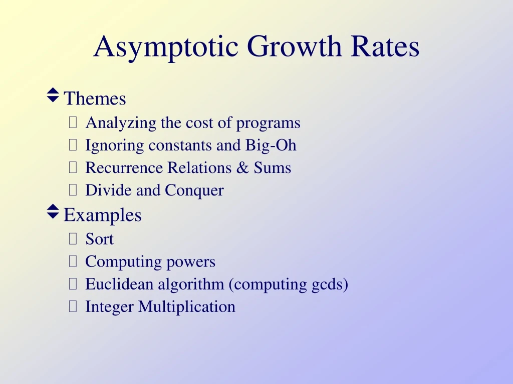
Asymptotic Growth Rates • Themes • Analyzing the cost of programs • Ignoring constants and Big-Oh • Recurrence Relations & Sums • Divide and Conquer • Examples • Sort • Computing powers • Euclidean algorithm (computing gcds) • Integer Multiplication
Asymptotic Growth Rates– “Big-O” (upper bound) • f(n) = O(g(n)) [f grows at the same rate or slower than g] iff: There exists positive constants c and n0 such that f(n) c g(n) for all n n0 • f is bound above by g • Note: Big-O does not imply a tight bound • Ignore constants and low order terms
Big-O, Examples • E.G. 1: 5n2 = O(n3) c = 1, n0= 5: 5n2 nn2 = n3 • E.G. 2: 100n2 = O(n2) c = 100, n0= 1 • E.G. 3: n3 = O(2n) c = 1, n0= 12 n3 (2n/3)3, n 2n/3 for n 12 [use induction]
Little-oLoose upper bound • f(n) = o(g(n)) [f grows strictly slower than g] f(n) = O(g(n)) and g(n) O(f(n)) • limn f(n)/g(n) = 0 • “f is bound above by g, but not tightly”
Little-o, restatement • limn f(n)/g(n) = 0 f(n) = o(g(n)) • >0, n0 s.t. n n0, f(n)/g(n) <
Equivalence - Theta • f(n) = (g(n)) [grows at the same rate] • f(n) = O(g(n)) and g(n) = O(f(n)) • g(n) = (f(n)) • limnf(n)/g(n) = c, c ≠ 0 f(n) = (g(n)) • “f is bound above by g, and below by g”
Common Results • [j < k] limn nj/nk = limn 1/n(k-j) = 0 • nj = o(nk), if j<k • [c < d] limn cn/dn = limn (c/d)n = 0 • cn = o(dn), if c<d • limn ln(n)/n = / • limn ln(n)/n = limn (1/n)/1 = 0 [L’Hopital’s Rule] • ln(n) = o(n) • [ > 0] ln(n) = o(n) [similar calculation]
Common Results • [c > 1, k an integer] limn nk/cn = / • limn knk-1/ cnln(c) • limn k(k-1)nk-2/ cnln(c)2 • … • limn k(k-1)…(k-1)/cnln(c)k = 0 • nk = o(cn)
Asymptotic Growth Rates • (log(n)) – logarithmic [log(2n)/log(n) = 1 + log(2)/log(n)] • (n) – linear [double input double output] • (n2) – quadratic [double input quadruple output] • (n3) – cubit [double input output increases by factor of 8] • (nk) – polynomial of degree k • (cn) – exponential [double input square output]
Asymptotic Manipulation • (cf(n)) = (f(n)) • (f(n) + g(n)) = (f(n)) if g(n) = O(f(n))
Computing Time Functions • Computing time function is the time to execute a program as a function of its inputs • Typically the inputs are parameterized by their size [e.g. number of elements in an array, length of list, size of string,…] • Worst case = max runtime over all possible inputs of a given size • Best case = min runtime over all possible inputs of a given size • Average = avg. runtime over specified distribution of inputs
Analysis of Running Time • We can only know the cost up to constants through analysis of code [number of instructions depends on compiler, flags, architecture, etc.] • Assume basic statements are O(1) • Sum over loops • Cost of function call depends on arguments • Recursive functions lead to recurrence relations
Loops and Sums • for (i=0;i<n;i++) • for (j=i;j<n;j++) • S; // assume cost of S is O(1)
Merge Sort and Insertion Sort • Insertion Sort • TI(n) = TI(n-1) + O(n) =(n2) [worst case] • TI(n) = TI(n-1) + O(1) =(n) [best case] • Merge Sort • TM(n) = 2TM(n/2) + O(n) =(nlogn) [worst case] • TM(n) = 2TM(n/2) + O(n) =(nlogn) [best case]
Karatsuba’s Algorithm • Using the classical pen and paper algorithm two n digit integers can be multiplied in O(n2) operations. Karatsuba came up with a faster algorithm. • Let A and B be two integers with • A = A110k + A0, A0 < 10k • B = B110k + B0, B0 < 10k • C = A*B = (A110k + A0)(B110k + B0) = A1B1102k + (A1B0 + A0 B1)10k + A0B0 Instead this can be computed with 3 multiplications • T0 = A0B0 • T1 = (A1 + A0)(B1 + B0) • T2 = A1B1 • C = T2102k + (T1 - T0 - T2)10k + T0
Complexity of Karatsuba’s Algorithm • Let T(n) be the time to compute the product of two n-digit numbers using Karatsuba’s algorithm. Assume n = 2k. T(n) = (nlg(3)), lg(3) 1.58 • T(n) 3T(n/2) + cn 3(3T(n/4) + c(n/2)) + cn = 32T(n/22) + cn(3/2 + 1) 32(3T(n/23) + c(n/4)) + cn(3/2 + 1) = 33T(n/23) + cn(32/22 + 3/2 + 1) … 3iT(n/2i) + cn(3i-1/2i-1 + … + 3/2 + 1) ... cn[((3/2)k - 1)/(3/2 -1)] --- Assuming T(1) c 2c(3k - 2k) 2c3lg(n) = 2cnlg(3)
Divide & Conquer Recurrence Assume T(n) = aT(n/b) + (n) • T(n) = (n) [a < b] • T(n) = (nlog(n)) [a = b] • T(n) = (nlogb(a)) [a > b]