Location
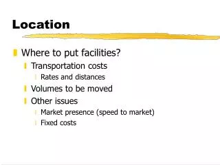
Location. Where to put facilities? Transportation costs Rates and distances Volumes to be moved Other issues Market presence (speed to market) Fixed costs. 1-Dimensional Intuition. Customers. -6. -5. -4. -3. -2. -1. 0. 1. 2. 3. 4. 5. 6. Where to locate?.

Location
E N D
Presentation Transcript
Location • Where to put facilities? • Transportation costs • Rates and distances • Volumes to be moved • Other issues • Market presence (speed to market) • Fixed costs
1-Dimensional Intuition Customers -6 -5 -4 -3 -2 -1 0 1 2 3 4 5 6 Where to locate?
1-Dimensional Intuition Customers -6 -5 -4 -3 -2 -1 0 1 2 3 4 5 6 Where to locate?
1-Dimensional Intuition Customers -6 -5 -4 -3 -2 -1 0 1 2 3 4 5 6 Where to locate?
1-Dimensional Intuition Customers -6 -5 -4 -3 -2 -1 0 1 2 3 4 5 6 Where to locate
What about “Weight” Weight 3 Customers -6 -5 -4 -3 -2 -1 0 1 2 3 4 5 6 Where to locate?
What about “Weight” Weight 2 Customers -6 -5 -4 -3 -2 -1 0 1 2 3 4 5 6 Where to locate?
2-Dimensional Location D 5 D 4 Manhattan Metric or L1 norm Distance 4 + 5 = 9
7 7 4 4 1 1 2 2 5 5 3 3 8 8 9 9 10 10 6 6 2-Dimensions • If all the points are the same “weight” D Y D D D Where to locate? X
D D D D 7 7 4 4 1 1 2 2 5 5 3 3 8 8 9 9 10 10 6 6 2-Dimensions • If all the points are the same “weight” Y Where to locate? X
D D D D D 4 7 1 7 4 2 5 1 3 2 5 3 8 9 8 9 6 10 10 6 2-Dimensions • Euclidean Distance or L2 norm • Successive Approximations: • X = Average of X’s • Y = Average of Y’s • Calculate distances d1, d2, ... • X = X1/d1+X2/d2+…X4/d4 • 1/d1 + 1/d2 + …1/d4 • Y = Y1/d1+Y2/d2+…Y4/d4 • 1/d1 + 1/d2 + …1/d4 • Repeat until movement is small Y X
D D D D
“Weights and Rates” • If there are • Different volumes V1, V2, …, V4 • Different transportation rates R1, R2, …, R4 associated with each location • Replace Xi with ViRiXi • Replace Yi with ViRiYi • (Not when calculating distances)
Over Emphasis • Useful for getting in the neighborhood • One or two iterations generally does this • Ignores lots of (important) details • Availability and cost of sites • Actual transportation network • Reality of freight rates • Non-linear • Often relatively insensitive to distance (LTL) • Dynamics of demand
Locating Many Facilities • Select a number of locations • Guess at initial positions • Assign Customers to those locations • Repeat: • Calculate best location to serve assigned customers • Calculate best customers to serve from those locations
Locate Distribution Centers • Based on Ford Auto Dealerships in Canada • Parts distribution • 4 Distribution Centers • Consider only distance to dealerships • Ignore volume (to keep it simple) • Illustrate approach • Compare with “Actual”
Mixed Integer Linear Programming • Does guarantee the quality of the solution • Computationally more demanding • More Flexible • Technically more demanding
Example 13.5 page 498 • 2 Products • 3 Customers • Single sourcing • 2 warehouses
Heuristics • Speed the MIP solution • Reduce computational demands • More interactive • No guarantee of optimality
Some Heuristics • Multiple Center of Gravity method for each number • Evaluate other costs after the fact • Inventory • Fixed Costs • Etc. • Successive Elimination • Successive Approximation
Successive Elimination • Illustrate with our MIP example • Replace the computationally demanding MIP with sequence of LPs
Successive Elimination • Both $ 3,150,000 • Remove 1 $ 3,050,000 • Remove 2 Not Feasible • With more choices, continue as long as costs reduce… • Does not always find optimum
Successive Approximation • Calculate an imputed cost per unit based on anticipated volume through each warehouse • Solve an LP to determine best volumes at these rates • Repeat • Calculate imputed costs per unit based on volumes • Calculate best volumes at imputed costs
Covering Models • Each site “covers” some customers • Select a best set of sites that cover all customers