Download
1 / 6
60 likes | 88 Vues
Learn about normal distributions and the standard normal distribution, including important concepts, characteristics, and examples. Discover how to find areas below the standard normal curve using practical methods and tables. Enhance your understanding of continuous random variables that follow a normal distribution and the significance of mean and standard deviation. This comprehensive guide provides insights into the standard normal distribution, its relationship with normally distributed variables, and techniques to determine cumulative areas and probabilities.

E N D
5.1 Introduction to Normal Distributions and the Standard Normal Distribution • Important Concepts: • Normal Distribution • Standard Normal Distribution • Finding Areas Below the Standard Normal Curve
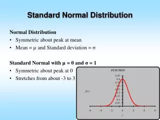
5.1 Introduction to Normal Distributions and the Standard Normal Distribution • What is a normal distribution? • A continuous probability distribution for a random variable X. • The graph of a normal distribution is called the normal curve. • The shape of a normal curve is determined by two parameters – the mean and the standard deviation of the random variable (see p. 235).
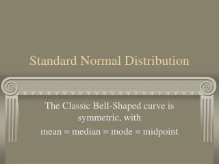
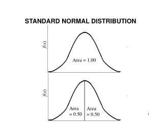
5.1 Introduction to Normal Distributions and the Standard Normal Distribution • If a variable is normally distributed, or follows a normal distribution, what does that tell us? • The mean, median, and mode of the variable are all equal. • The normal curve is bell-shaped and is symmetric about the mean. • The total area below the normal curve is 1. • The tails of the normal curve are asymptotic to the x-axis. • Inflection points are located one standard deviation away from the mean.
5.1 Introduction to Normal Distributions and the Standard Normal Distribution • Examples of continuous random variables that are normally distributed, i.e., follow a normal distribution: • The heights and weights of adult males and females • The body temperatures of rats • The cholesterol levels of adults • Intelligence Quotients (IQ Scores) • Life spans of light bulbs • Weights of newborn infants
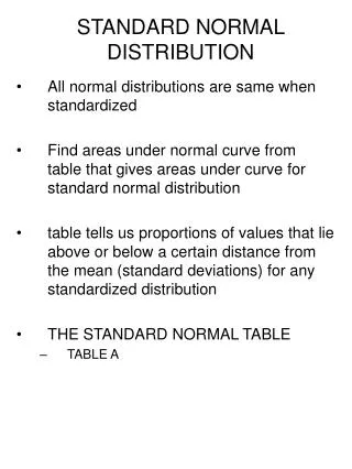
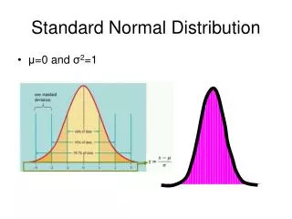
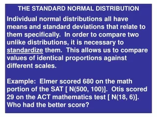
5.1 Introduction to Normal Distributions and the Standard Normal Distribution • The standard normal distribution is a normal distribution with a mean of 0 and a standard deviation of 1. • Very important relationship we will need later: • If X is a normally distributed variable with mean µ and standard deviation σ, then the variable follows the standard normal distribution.
5.1 Introduction to Normal Distributions and the Standard Normal Distribution • Finding areas below the standard normal curve. • We use Table 4 to find cumulative areas #18 p. 243 (area to the left) #26* (area to the left) #20 (area to the right) #32 (area between two values) • Standard normal curves and probabilities #48 p. 245 #54 #56