5.1 Intro to Normal Distributions
170 likes | 625 Vues
5.1 Intro to Normal Distributions. Statistics Mrs. Spitz Fall 2008. Objectives/Assignment. How to interpret graphs of normal probability distributions How to find areas under a normal curve, and use them to find probabilities for random variables with normal distributions.

5.1 Intro to Normal Distributions
E N D
Presentation Transcript
5.1 Intro to Normal Distributions Statistics Mrs. Spitz Fall 2008
Objectives/Assignment • How to interpret graphs of normal probability distributions • How to find areas under a normal curve, and use them to find probabilities for random variables with normal distributions. • Assn: pp. 198-201 #1-26 all
Properties of a Normal Distribution • In 4.1, we learned that a continuous random variable has an infinite number of values that can be represented by an interval on the number line. It’s probability distribution is called a continuous probability distribution. In this chapter, we will be studying the most important continuous probability distribution in statistics—the normal distribution.
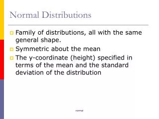
Guidelines: Properties of a Normal Distribution • A normal distribution is a continuous probability distribution for a random variable, x. The graph of a normal distribution is called the normal curve. A normal distribution has the following properties. • The mean, median and mode are equal. • The normal curve is bell-shaped and is symmetric about the mean.
Guidelines: Properties of a Normal Distribution 3. The total area under the normal curve is equal to 1. 4. The normal curve approaches, but never touches the x-axis as it extends farther and farther away from the mean. 5. Between - and + (in the center of the curve) the graph curves downward. The graph curves upward to the left of - and to the right of + . The points at which the curve changes from curving upward to curving downward are called inflection points.
Guidelines: Properties of a Normal Distribution Inflection points
Guidelines: Properties of a Normal Distribution • A normal distribution can have any mean and any positive standard deviation. These two parameters, and completely determine the shape of a normal curve. The mean gives the location of the line of symmetry and the standard deviation describes how much the data are spread out.
Look at the three examples below: See the line of symmetry for each? That’s the mean. However, if it is fatter, then the standard deviation is greater. That’s the difference.
Ex. 1: Understanding Mean & Standard Deviation • Which normal curve has a greater mean? • Which normal curve has a greater standard deviation? SOLUTION: 1. The line of symmetry of curve A occurs at x = 15. The line of symmetry of curve B occurs at x = 12. So, curve A has a greater mean.
Ex. 1: Understanding Mean & Standard Deviation • Which normal curve has a greater mean? • Which normal curve has a greater standard deviation? SOLUTION: 2. Curve B is more spread out than curve A, so curve B has a greater standard deviation.
Try it yourself: • Consider the normal curves shown below. Which normal curve has the greatest mean? Which normal curve has the greatest standard deviation? Justify your answers? • Find the location of the line of symmetry for each curve. Make a conclusion about which mean is greatest. • Determine which normal curve is more spread out. Make a conclusion about which standard deviation is the greatest.
Try it yourself: 1a. A: 45, B: 60, C: 45 1b. C has the most spread, so the greatest standard deviation Slide 11B
Ex 2: Interpreting graphs of Normal Distributions • The heights (in feet) of fully grown white oak trees are normally distributed. The normal curve shown below represents this distribution. What is the mean height of a fully grown white oak tree? Estimate the standard deviation of this normal distribution. Mean of about 90 feet with standard deviation of about 3.5 feet.
Normal Curves and Probability • The total area under a probability curve is equal to 1. The area of a region under a probability curve gives the probability that the random variable will have a value in the corresponding interval. In this chapter, you will learn several ways to find areas, under normal curves. You have already studied one of these ways in section 2.4—The Empirical Rule.
115 70 85 100 130 Ex. 3: Estimating a Probability for a Normal Curve • Adult IQ scores are normally distributed with = 100 and = 15. Estimate the probability that a randomly chosen adult has an IQ between 70 and 115. Solution: Draw the curve. Using the Empirical Rule, the area under the normal curve between these two values is: Area = .135 + .34 + .34 = .815. So the probability the adult has an IQ between 70 and 115 is about .815.