Download

1 / 45
460 likes | 628 Vues
The greatest blessing in life is in giving and not taking. 1-Way Anova. 1. One-Way Analysis of Variance. Y= DEPENDENT VARIABLE (“yield”) (“response variable”) (“quality indicator”) X = INDEPENDENT VARIABLE (A possibly influential FACTOR). 2.

E N D
The greatest blessing in life is in giving and not taking. 1-Way Anova 1 1-Way ANOVA
One-Way Analysis of Variance Y= DEPENDENT VARIABLE (“yield”) (“response variable”) (“quality indicator”) X = INDEPENDENT VARIABLE (A possibly influential FACTOR) 2
OBJECTIVE: To determine the impact of X on Y Mathematical Model: Y = f (x, ) , where = (impact of) all factors other than X Ex: Y = Battery Life (hours) X = Brand of Battery = Many other factors (possibly, some we’re unaware of)
Completely Randomized Design (CRD) • Goal: to study the effect of Factor X • The same # of observations are taken randomly and independently from the individuals at each level of Factor X • i.e. n1=n2=…nc (c levels) 1-Way ANOVA 4
1 2 3 4 5 6 7 8 1.8 4.2 8.6 7.0 4.2 4.2 7.8 9.0 5.0 5.4 4.6 5.0 7.8 4.2 7.0 7.4 1.0 4.2 4.2 9.0 6.6 5.4 9.8 5.8 5.8 2.6 4.6 5.8 7.0 6.2 4.6 8.2 7.4 Example: Y = LIFETIME (HOURS) BRAND 3 replications per level 1-Way ANOVA 5
Analysis of Variance 1-Way ANOVA 6
StatisticalModel C “levels” OF BRAND R observations for each level 1 2 • • • • • • • • R 1 2 • • • • C Y11 Y12 • • • • • • •Y1R Yij = + i + ij i = 1, . . . . . , C j = 1, . . . . . , R Y21 • • • • • • YcI • • • • • Yij YcR • • • • • • • • 1-Way ANOVA 7
Where = OVERALL AVERAGE i = index for FACTOR (Brand) LEVEL j= index for “replication” i = Differential effect associated with ith level of X (Brand i) = mi – m and ij = “noise” or “error” due to other factors associated with the (i,j)th data value. mi = AVERAGE associated with ith level of X (brand i) m= AVERAGE of mi ’s. 1-Way ANOVA 8
Yij = + i + ij By definition, i = 0 C i=1 The experiment produces R x C Yij data values. The analysis produces estimates of ,c. (We can then get estimates of the ij by subtraction). 1-Way ANOVA 9
Let Y1, Y2, etc., be level means Y • = Y i /C = “GRAND MEAN” (assuming same # data points in each column) (otherwise, Y • = mean of all the data) c i=1 1-Way ANOVA 10
MODEL: Yij = + i + ij Y• estimates Yi - Y • estimatesi (= mi – m) (for all i) These estimates are based on Gauss’ (1796) PRINCIPLE OF LEAST SQUARES and on COMMON SENSE 1-Way ANOVA 11
MODEL: Yij = + j + ij If you insert the estimates into the MODEL, (1) Yij = Y • + (Yj - Y • ) + ij. < it follows that our estimate of ij is (2) ij = Yij – Yj, called residual < 1-Way ANOVA 12
Then, Yij = Y• + (Yi - Y• ) + ( Yij - Yi) or, (Yij - Y• ) = (Yi - Y•) + (Yij - Yi ) { { { (3) Variability in Y associated with all other factors Variability in Y associated with X TOTAL VARIABILITY in Y + = 1-Way ANOVA 13
If you square both sides of (3), and double sum both sides (over i and j), you get, [after some unpleasant algebra, but lots of terms which “cancel”] {{ C C R C R (Yij - Y• )2 = R • (Yi - Y•)2 + (Yij - Yi)2 { i=1 i=1 j=1 i=1 j=1 ( SSW (SSE) SUM OF SQUARES WITHIN SAMPLES TSS TOTAL SUM OF SQUARES SSB SUM OF SQUARES BETWEEN SAMPLES + + = = ( ( ( ( ( 1-Way ANOVA 14
ANOVA TABLE SOURCE OF VARIABILITY Mean square (M.S.) SSQ DF Between samples (due to brand) SSB SSB C - 1 = MSB C - 1 Within samples (due to error) SSW MSW = (R - 1) • C SSW (R-1)•C TOTAL TSS RC -1 1-Way ANOVA 15
1 2 3 4 5 6 7 8 1.8 4.2 8.6 7.0 4.2 4.2 7.8 9.0 5.0 5.4 4.6 5.0 7.8 4.2 7.0 7.4 1.0 4.2 4.2 9.0 6.6 5.4 9.8 5.8 5.8 2.6 4.6 5.8 7.0 6.2 4.6 8.2 7.4 Example: Y = LIFETIME (HOURS) BRAND 3 replications per level SSB= 3 ( [2.6 - 5.8]2 + [4.6 - 5.8] 2+ • • • + [7.4 - 5.8]2) = 3 (23.04) = 69.12 1-Way ANOVA 16
SSW =? (1.8 - 2.6)2 = .64 (4.2 - 4.6)2 =.16 (9.0 -7.4)2 = 2.56 (5.0 - 2.6)2 = 5.76 (5.4 - 4.6)2= .64 • • • • (7.4 - 7.4)2 = 0 (1.0 - 2.6)2 = 2.56 (4.2 - 4.6)2= .16 (5.8 - 7.4)2 = 2.56 8.96 .96 5.12 Total of (8.96 + .96 + • • • + 5.12), SSW = 46.72 1-Way ANOVA 17
ANOVA TABLE Source of Variability df M.S. SSQ 7 = 8 - 1 69.12 BRAND 9.87 ERROR 2.92 16 = 2 (8) 46.72 TOTAL 115.84 23 = (3 • 8) -1 1-Way ANOVA 18
We can show: “VCOL” { E (MSB) = 2+ MEASURE OF DIFFERENCES AMONG LEVEL MEANS ( R ( • (i - )2 { C-1 i E (MSW) = 2 (Assuming Yij follows N(j , 2) and they are independent) 1-Way ANOVA 19
E ( MSBC ) = 2 +VCOL E ( MSW) = 2 This suggests that There’s some evidence of non-zero VCOL, or “level of X affects Y” if MSBC > 1 , MSW if MSBC No evidence that VCOL > 0, or that “level of X affects Y” < 1 , MSW 1-Way ANOVA 20
With HO: Level of X has no impact on Y HI: Level of X does have impact on Y, We need MSBC > > 1 MSW to reject HO. 1-Way ANOVA 21
More Formally, HO: 1 = 2 = • • • c = 0 HI: not all j = 0 OR (All level means are equal) HO: 1 = 2 = • • • • c HI: not all j are EQUAL 1-Way ANOVA 22
The distribution of MSB = “Fcalc” , is MSW The F - distribution with (C-1, (R-1)C) degrees of freedom Assuming HO true. C = Table Value 1-Way ANOVA 23
In our problem: ANOVA TABLE Source of Variability M.S. Fcalc SSQ df 7 69.12 BRAND 9.87 3.38 ERROR 2.92 = 9.87 2.92 16 46.72 1-Way ANOVA 24
F table: table 8 = .05 C = 2.66 3.38 (7,16 DF) 1-Way ANOVA 25
Hence, at = .05, Reject Ho . (i.e., Conclude that level of BRAND does have an impact on battery lifetime.) 1-Way ANOVA 26
MINITAB INPUT life brand 1.8 1 5.0 1 1.0 1 4.2 2 5.4 2 4.2 2 . . . . . . 9.0 8 7.4 8 5.8 8 1-Way ANOVA 27
ONE FACTOR ANOVA (MINITAB) MINITAB: STAT>>ANOVA>>ONE-WAY Analysis of Variance for life Source DF SS MS F P brand 7 69.12 9.87 3.38 0.021 Error 16 46.72 2.92 Total 23 115.84 Estimate of the common variances^2 1-Way ANOVA 28
1-Way ANOVA 29
Assumptions MODEL: Yij = + i + ij 1.) the ij are indep. random variables 2.) Each ij is Normally Distributed E(ij) = 0 for all i, j 3.) 2(ij) = constant for all i, j Run order plot Normality plot & test Residual plot & test 1-Way ANOVA 30
Diagnosis: Normality • The points on the normality plot must more or less follow a line to claim “normal distributed”. • There are statistic tests to verify it scientifically. • The ANOVA method we learn here is not sensitive to the normality assumption. That is, a mild departure from the normal distribution will not change our conclusions much. Normal probability plot & normality test of residuals 1-Way ANOVA 31
Minitab: stat>>basic statistics>>normality test 1-Way ANOVA 32
Diagnosis: Constant Variances • The points on the residual plot must be more or less within a horizontal band to claim “constant variances”. • There are statistic tests to verify it scientifically. • The ANOVA method we learn here is not sensitive to the constant variances assumption. That is, slightly different variances within groups will not change our conclusions much. Tests and Residual plot: fitted values vs. residuals 1-Way ANOVA 33
Minitab: Stat >> Anova >> One-way 1-Way ANOVA 34
Minitab: Stat>> Anova>> Test for Equal variances 1-Way ANOVA 35
Diagnosis: Randomness/Independence • The run order plot must show no “systematic” patterns to claim “randomness”. • There are statistic tests to verify it scientifically. • The ANOVA method is sensitive to the randomness assumption. That is, a little level of dependence between data points will change our conclusions a lot. Run order plot: order vs. residuals 1-Way ANOVA 36
Minitab: Stat >> Anova >> One-way 1-Way ANOVA 37
KRUSKAL - WALLIS TEST (Non - Parametric Alternative) HO: The probability distributions are identical for each level of the factor HI: Not all the distributions are the same 1-Way ANOVA 38
Brand ABC 32 32 28 30 32 21 30 26 15 29 26 15 26 22 14 23 20 14 20 19 14 19 16 11 18 14 9 12 14 8 BATTERY LIFETIME (hours) (each column rank ordered, for simplicity) Mean: 23.9 22.1 14.9 (here, irrelevant!!) 1-Way ANOVA 39
HO: no difference in distribution among the three brands with respect to battery lifetime HI: At least one of the 3 brands differs in distribution from the others with respect to lifetime 1-Way ANOVA 40
Ranks in ( ) Brand ABC 32 (29) 32 (29) 28 (24) 30 (26.5) 32 (29) 21 (18) 30 (26.5) 26 (22) 15 (10.5) 29 (25) 26 (22) 15 (10.5) 26 (22) 22 (19) 14 (7) 23 (20) 20 (16.5) 14 (7) 20 (16.5) 19 (14.5) 14 (7) 19 (14.5) 16 (12) 11 (3) 18 (13) 14 (7) 9 (2) 12 (4) 14 (7) 8 (1) T1 = 197T2 = 178 T3 = 90 n1 = 10 n2 = 10 n3 = 10 1-Way ANOVA 41
TEST STATISTIC: K 12 • (Tj2/nj ) - 3 (N + 1) H = N (N + 1) j = 1 nj = # data values in column j N = nj K = # Columns (levels) Tj = SUM OF RANKS OF DATA ON COL j When all DATA COMBINED (There is a slight adjustment in the formula as a function of the number of ties in rank.) K j = 1 1-Way ANOVA 42
H = [ 12 197 2 178 2 902 30 (31) 10 10 10 [ + + - 3 (31) = 8.41 (with adjustment for ties, we get 8.46) 1-Way ANOVA 43
c21-adf = .05 = F1-adf, df 5.99 8.41 = H What do we do with H? We can show that, under HO , H is well approximated by a 2 distribution with df = K - 1. Here, df = 2, and at = .05, the critical value = 5.99 8 Reject HO; conclude that mean lifetime NOT the same for all 3 BRANDS 1-Way ANOVA 44
Minitab: Stat >> Nonparametrics >> Kruskal-Wallis • Kruskal-Wallis Test: life versus brand • Kruskal-Wallis Test on life • brand N Median AveRank Z • 1 3 1.800 4.5 -2.09 • 2 3 4.200 7.8 -1.22 • 3 3 4.600 11.8 -0.17 • 4 3 7.000 16.5 1.05 • 5 3 6.600 13.3 0.22 • 6 3 4.200 7.8 -1.22 • 7 3 7.800 20.0 1.96 • 8 3 7.400 18.2 1.48 • Overall 24 12.5 • H = 12.78 DF = 7 P = 0.078 • H = 13.01 DF = 7 P = 0.072 (adjusted for ties) 1-Way ANOVA 45