Multi-way Anova
Multi-way Anova. Identifying and quantifying sources of variation Ability to "factor out" certain sources - ("adjusting") For the beginning, we will reproduce paired t-test results by assuming that arrays are one of the factors in a Two-way ANOVA


Multi-way Anova
E N D
Presentation Transcript
Multi-way Anova • Identifying and quantifying sources of variation • Ability to "factor out" certain sources - ("adjusting") • For the beginning, we will reproduce paired t-test results by assuming that arrays are one of the factors in a Two-way ANOVA • Second, adjusting for the dye effects in a Three-way ANOVA • Third, four and more - way ANOVA when having multiple factors of interest
Statistical Model Parameter Estimates Null Hypotheses Null Distributions Statistical Inference in Two-way ANOVA
No-intercept Model Null Hypotheses Null Distributions Alternative Formulations of the Two-way ANOVA • Parameter Estimates • Gets complicated • Regardless of how the model is parametrized certain parametersremain unchanged (Trt2-Trt1) • In this sense all formulations are equivalent
Re-organizing data for ANOVA > DAnova<-NNBLimmadataC > DAnova$weights<-cbind(DAnova$weights,DAnova$weights) > DAnova$M<-cbind((DAnova$A+DAnova$M/2),DAnova$A-(DAnova$M/2)) > DAnova$A<-cbind(DAnova$A,DAnova$A) > attributes(DAnova) $names [1] "weights" "targets" "genes" "printer" "M" "A" $class [1] "MAList" attr(,"package") [1] "limma" > NNBLimmadataC$M[1,] 51-C1-3-vs-W1-5 60-W2-3-vs-C2-5 72-C3-3-vs-W3-5 79-W4-3-vs-C4-5 82-C5-3-vs-W5-5 97-W6-3-vs-C6-5 -0.05280598 -0.15767422 0.40130216 -0.35292771 -0.22061576 -0.21653047 > NNBLimmadataC$A[1,] 51-C1-3-vs-W1-5 60-W2-3-vs-C2-5 72-C3-3-vs-W3-5 79-W4-3-vs-C4-5 82-C5-3-vs-W5-5 97-W6-3-vs-C6-5 6.289658 6.129577 6.483613 6.452317 6.510143 7.106134 > DAnova$M[1,] 51-C1-3-vs-W1-5 60-W2-3-vs-C2-5 72-C3-3-vs-W3-5 79-W4-3-vs-C4-5 82-C5-3-vs-W5-5 97-W6-3-vs-C6-5 6.263255 6.050740 6.684264 6.275853 6.399835 6.997869 51-C1-3-vs-W1-5 60-W2-3-vs-C2-5 72-C3-3-vs-W3-5 79-W4-3-vs-C4-5 82-C5-3-vs-W5-5 97-W6-3-vs-C6-5 6.316061 6.208414 6.282962 6.628781 6.620451 7.214399
Setting-up the design matrix for limma > targets SlideNumber FileName Cy3 Cy5 Date 51-C1-3-vs-W1-5 51 51-C1-3-vs-W1-5.gpr C W 11/8/2004 60-W2-3-vs-C2-5 60 60-W2-3-vs-C2-5.gpr W C 11/8/2004 72-C3-3-vs-W3-5 72 72-C3-3-vs-W3-5.gpr C W 11/8/2004 79-W4-3-vs-C4-5 79 79-W4-3-vs-C4-5.gpr W C 11/8/2004 82-C5-3-vs-W5-5 82 82-C5-3-vs-W5-5.gpr C W 11/8/2004 97-W6-3-vs-C6-5 97 97-W6-3-vs-C6-5.gpr W C 11/8/2004 > trt<-c(targets$Cy5,targets$Cy3) > trt [1] "W" "C" "W" "C" "W" "C" "C" "W" "C" "W" "C" "W" > array<-c(1:6,1:6) > array [1] 1 2 3 4 5 6 1 2 3 4 5 6
Setting-up the design matrix for limma > designa<-model.matrix(~-1+factor(array)+factor(trt)) > designa factor(array)1 factor(array)2 factor(array)3 factor(array)4 factor(array)5 factor(array)6 factor(trt)W 1 1 0 0 0 0 0 1 2 0 1 0 0 0 0 0 3 0 0 1 0 0 0 1 4 0 0 0 1 0 0 0 5 0 0 0 0 1 0 1 6 0 0 0 0 0 1 0 7 1 0 0 0 0 0 0 8 0 1 0 0 0 0 1 9 0 0 1 0 0 0 0 10 0 0 0 1 0 0 1 11 0 0 0 0 1 0 0 12 0 0 0 0 0 1 1 attr(,"assign") [1] 1 1 1 1 1 1 2 attr(,"contrasts") attr(,"contrasts")$"factor(array)" [1] "contr.treatment" attr(,"contrasts")$"factor(trt)" [1] "contr.treatment"
Setting-up the design matrix for limma > colnames(designa)<-c(paste("A",1:6,sep=""),"W") > designa A1 A2 A3 A4 A5 A6 W 1 1 0 0 0 0 0 1 2 0 1 0 0 0 0 0 3 0 0 1 0 0 0 1 4 0 0 0 1 0 0 0 5 0 0 0 0 1 0 1 6 0 0 0 0 0 1 0 7 1 0 0 0 0 0 0 8 0 1 0 0 0 0 1 9 0 0 1 0 0 0 0 10 0 0 0 1 0 0 1 11 0 0 0 0 1 0 0 12 0 0 0 0 0 1 1 attr(,"assign") [1] 1 1 1 1 1 1 2 attr(,"contrasts") attr(,"contrasts")$"factor(array)" [1] "contr.treatment" attr(,"contrasts")$"factor(trt)" [1] "contr.treatment"
Comparing to paired t-test > Anova<-lmFit(DAnova,designa) > > Anova$coefficients[2,] A1 A2 A3 A4 A5 A6 W 8.36197475 9.90627295 11.34002704 10.77586480 9.35096212 9.92299117 -0.03068036 > LimmaPTT$coefficients[2] [1] -0.03068036 > Anova$coefficients[1,] A1 A2 A3 A4 A5 A6 W NA NA 6.3898451 6.3585492 6.4163747 7.0123661 0.1875361 > LimmaPTT$coefficients[1] [1] 0.1875361 >
Comparing to paired t-test > plot(Anova$coefficients[,"W"],LimmaPTT$coefficients) > plot(Anova$sigma,LimmaPTT$sigma) > plot(Anova$stdev.unscaled[,"W"],LimmaPTT$stdev.unscaled) > plot(Anova$sigma*Anova$stdev.unscaled[,"W"],LimmaPTT$sigma*LimmaPTT$stdev.unscaled) > plot(Anova$df.residual,LimmaPTT$df.residual)
Adjusting for Dye - Three-way ANOVA > dye<-c(rep("Cy5",6),rep("Cy3",6)) > > designad<-model.matrix(~-1+factor(array)+factor(dye)+factor(trt)) > #designad > colnames(designad)<-c(paste("A",1:6,sep=""),"Cy5","W") > designad A1 A2 A3 A4 A5 A6 Cy5 W 1 1 0 0 0 0 0 1 1 2 0 1 0 0 0 0 1 0 3 0 0 1 0 0 0 1 1 4 0 0 0 1 0 0 1 0 5 0 0 0 0 1 0 1 1 6 0 0 0 0 0 1 1 0 7 1 0 0 0 0 0 0 0 8 0 1 0 0 0 0 0 1 9 0 0 1 0 0 0 0 0 10 0 0 0 1 0 0 0 1 11 0 0 0 0 1 0 0 0 12 0 0 0 0 0 1 0 1 attr(,"assign") [1] 1 1 1 1 1 1 2 3 attr(,"contrasts") attr(,"contrasts")$"factor(array)" [1] "contr.treatment" attr(,"contrasts")$"factor(dye)" [1] "contr.treatment" attr(,"contrasts")$"factor(trt)" [1] "contr.treatment"
Adjusting for Dye - Three-way ANOVA >Anovad<-lmFit(DAnova,designad) > > Anova$coefficients[2,] A1 A2 A3 A4 A5 A6 W 8.36197475 9.90627295 11.34002704 10.77586480 9.35096212 9.92299117 -0.03068036 > LimmaPTT$coefficients[2] [1] -0.03068036 > Anovad$coefficients[2,] A1 A2 A3 A4 A5 A6 Cy5 W 8.38440701 9.92870520 11.36245930 10.79829705 9.37339438 9.94542342 -0.04486451 -0.03068036 > Anova$coefficients[1,] A1 A2 A3 A4 A5 A6 W NA NA 6.3898451 6.3585492 6.4163747 7.0123661 0.1875361 > LimmaPTT$coefficients[1] [1] 0.1875361 > Anovad$coefficients[1,] A1 A2 A3 A4 A5 A6 Cy5 W NA NA 6.43844153 6.40714571 6.46497115 7.06096259 -0.09719295 0.18753615 >
Comparing to paired t-test > plot(Anovad$coefficients[,"W"],LimmaPTT$coefficients) > plot(Anovad$sigma,LimmaPTT$sigma) > plot(Anovad$stdev.unscaled[,"W"],LimmaPTT$stdev.unscaled) > plot(Anovad$sigma*Anova$stdev.unscaled[,"W"],LimmaPTT$sigma*LimmaPTT$stdev.unscaled) > plot(Anovad$df.residual,LimmaPTT$df.residual)
Comparing to paired t-test > AnovaB<-eBayes(Anova) > AnovadB<-eBayes(Anovad) > volcanoplot(AnovaB,coef=7) > volcanoplot(AnovadB,coef=8)