Analysis of Variance or ANOVA
380 likes | 590 Vues
Analysis of Variance or ANOVA. In ANOVA, we are interested in comparing the means of different populations (usually more than 2 populations).

Analysis of Variance or ANOVA
E N D
Presentation Transcript
In ANOVA, we are interested in comparing the means of different populations (usually more than 2 populations). Since this technique has frequently been applied to medical research, samples from the different populations are referred to as different treatment groups.
Main Idea behind Analysis of Variance • Measure the variability within the treatment groups and also the variability between the treatment groups. • The “between” variability is due to both differences in treatment and the random error component. • The “within” variability is due only to the random error component. • So, if there are significant treatment differences, the “between” variability should be substantially larger than the “within” variability.
In ANOVA, the null hypothesis H0 is always essentially “there are no differences in treatment” and the alternative hypothesis H1 is always essentially “there is a difference in treatment.” If the problem says “test whether there are no treatment effects,” H0 is “there are NO differences in treatment.” If the problem says “test whether there are treatment effects,” H0 is “there are NO differences in treatment.”
We will begin with one-factor ANOVA. Suppose we’re looking at the effects of different types of heart medication on pulse rate. An individual’s pulse rate is the sum of different effects. If there is no difference in the effects of the various heart medications or treatments, then the middle effect above is zero. That is what we would like to test.
Example 1: A manager is comparing the output of 3 machines. He has recorded 5 randomly selected minutes of operation for machine 1, 10 minutes for machine 2, and 6 minutes for machine 3. The output is as shown below.
In this example, we have n = # of observations = 21 and c = # of groups (or # of machines here) = 3
We compute the mean output per minute for each machine. The grand mean for all the machines combined is (42+67+64)/21 = 8.238.
We next look at the variation in output by computing sums of squared deviations.
The sum of squared variation within groups or SS withinis the sum of the sums of squared deviations for the 3 groups = 27.2 + 30.10 + 15.33 = 72.63 .
The mean squared variation within groups MS within = (SS Within) / (n – c). = 72.63/(21 – 3) = 72.63/18 = 4.035
The sum of squared variation between groups or SS Between is The mean square variation between groups or MS Between is In our example, n1=5 n2=10 n3=6 c = 3
The sum of squares total or SS Total= SS Between + SS Within The mean squared total or MS Total= SS Total /( n – 1)
We compile our information in a table called an ANOVA table. Notice that the degrees of freedom column adds up to the total at the bottom, and the sum of squares column adds up to the total at the bottom, but the mean square column does NOT add up to the total at the bottom.
Remember that the purpose of all the work we have been doing is to test whether there is a “treatment effect,” that is a difference in the means of the various groups. The hypotheses are H0: there is no difference in the means, and H1: there is a difference in the means. In our current example, we want to know if there is a difference in the mean output level of the various machines.
The statistic we use here is the F-statistic: The subscripts are the degrees of freedom of the F-statistic and they are the degrees of freedom that are associated with the numerator and the denominator of the statistic.
Like the 2, the F distribution is skewed to the right, and the critical region for the test is the right tail. f(Fc-1,n-c) acceptance region crit. reg. Fc-1, n-c
f(F2,18) acceptance region 0.05 crit. reg. F2, 18 3.55 For our current example, we have: The F table shows that for 2 and 18 degrees of freedom, the 5% critical value is 3.55. Since our F has a value of 7.33, we reject the null hypothesis and conclude that there is a difference in the mean output levels of the 3 machines. 7.33
Example 2: In order to compare the average tread life of 3 brands of tires, random samples of 6 tires of each brand are tested on a machine which simulates road conditions. The tread life for each tire is measured. Complete the analysis of variance table and test at the 1% level whether there is a difference in the average tread life of the 3 tire brands.
First we can calculate SS Total by adding SS Between and SS Within.
The degrees of freedom for the SS Between is c – 1 = 3 – 1 = 2, since there are three groups (3 tire brands).
The degrees of freedom for the SS Within is n – c = 18 – 3 = 15, since there are 18 observations (6 of each of the 3 brands).
The degrees of freedom for the SS total is n – 1 = 18 – 1 = 17.
The MS Between is (SS Between) / (dof Between) = 224.78 / 2 = 112.39
The MS Within is (SS Within) / (dof Within) = 118.83 / 15 = 7.922
The MS Total is (SS Total ) / (dof Total ) = 343.61 / 17 = 20.212
f(F2,15) acceptance region 0.01 crit. reg. F2, 15 6.36 So, The F table shows that for 2 and 15 degrees of freedom, the 1% critical value is 6.36. Since our F has a value of 14.19, we reject the null hypothesis and conclude that there is a difference in the mean tread life of the 3 tire brands. 14.19
Two-Factor ANOVA with Interaction Effects Now, we have two factors of interest, A and B, and the factors may interact to influence a particular variable Y with which we are concerned. For example, we may want to explore the effects of different teachers and different teaching methods on student performance. So,
We have 3 sets of hypotheses. • H0: factor A has no effect on Y. • H1: factor A has an effect on Y. • H0: factor B has no effect on Y. • H1: factor B has an effect on Y. • H0: the interaction of factors A and B has no effect on Y. • H1: the interaction of factors A and B has an effect on Y.
For each A and B possibility, we have r replications (or observations). • For example, suppose we have a = 4 different teachers, b = 3 different methods, and r = 3 replications. • There are 12 different teaching possibilities: You could have teacher A, B, C, or D, and that instructor could be using method 1, 2, or 3. • For each one of these 12 situations, we have 3 replications, or 3 observations, or exam scores of 3 students.
Test Statistics for Two-Way ANOVA Testing for the effect of factor A: Notice that in all three cases, the denominator is the same; it’s the Mean Squared Error. Testing for the effect of factor B: Testing for the effect of the interaction of A and B:
Example 3: Consider the following ANOVA table relating student performance to 4 teachers, 3 teaching methods, and the interaction of those 2 factors, using 3 replications.
Complete the table and then test at the 5% level whether student performance depends on (1) the teacher, (2) the teaching method, and (3) the interaction of the teacher and the method.
f(F3,24) acceptance region 0.05 crit. reg. F3, 24 3.01 Now we test the hypotheses. We’ll begin with the teachers. From the F table, we find that the 5% critical value for 3 and 24 degrees of freedom is 3.01. Since our statistic, 2.00, is in the acceptance region, we accept H0 that the teacher has no effect on student performance. 2.00
f(F2,24) acceptance region 0.05 crit. reg. F2, 24 3.40 Next we look at the teaching methods. From the F table, we find that the 5% critical value for 2 and 24 degrees of freedom is 3.40. Since our statistic, 4.00, is in the critical region, we reject H0 and accept H1 that the method does affect student performance. 4.00
f(F6,24) acceptance region 0.05 crit. reg. F6, 24 2.51 Last we look at the interaction of teachers and methods. From the F table, we find that the 5% critical value for 6 and 24 degrees of freedom is 2.51. Since 3 is in the critical region, we reject H0 & accept H1: there is an interaction effect of teacher & method on student performance. 3.00