Comprehensive Guide to Probability Theory Fundamentals

1. Probability theory Petter Mostad 2005.09.15

2. Sample space • The set of possible outcomes you consider for the problem you look at • You subdivide into different outcomes only as far as is relevant for your problem • The sample space is the start of a simplified model for reality • Events are subsets of the sample space

3. Set theory • The complement of subset is denoted • The intersection of and is denoted • The union of and is denoted • and are called mutually exclusive or disjoint if where is the empty set • If are subsets of a sample space , then they are called collectively exhaustive if

4. Venn diagrams

5. Computations with sets Examples of rules you can prove: • If are mutually exclusive and collectively exhaustive, then

6. Events as subsets • The union of events corresponds to ”or”, the intersection to ”and”, and the complement to ”not”. Examples: • A : The patient is given drug X • B : The patient dies • : The patient is given drug X and dies • : The patient is given drug X or s/he dies or both • : The patient does not die • : The patient is not given drug X, and dies

7. Definitions of probability • If A is a set of outcomes of an experiment, and if when repeating this experiment many times the frequency of A approaches a limit p, then the probability of A is said to be p. Or: • The probability of A is your ”belief” that A is true or will happen: It is an attribute of your knowledge about A. Over time, events given probability p should happen with frequency p.

8. Properties of probabilities • When probabilities are assigned to all outcomes in a sample space, such that • All probabilities are positive or zero. • The probabilities add up to one. then we say we have a probability model • The probability of an event A is the sum of the probabilities of the outcomes in A, and is written P(A)

9. Computations with probabilities Some consequences of the set-theory results: • When and are mutually exclusive, • In general,

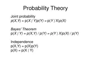
10. Conditional probability • If some information limits the sample space to a subset A, the relative probabilities for outcomes in A are the same, but they are scaled up so that they sum to 1. • We write P(B|A) for the probability of event B given event A. • In symbols:

11. The law of total probability • As and are disjoint, we get • Together with the definition of conditional probability, this gives the law of total probability:

12. Statistical independence • If P(B|A)=P(B), we say that B is statistically independent of A. • We can easily see that this happens if and only if • Thus B is statistically independent of A if and only if A is statistically independent of B.

13. Bayes theorem • Bayes theorem says that: • This can be deduced simply from definition of conditional probability: • Together with the law of total probability:

14. Example • A disease X has a prevalence of 1%. A test for X exists, and • If you are ill, the test is positive in 90% of cases • If you are not ill, the test is positive in 10% of cases. • You have a positive test: What is the probability that you have X?

15. Joint and marginal probabilities Assume are mutually exclusive and collectively exhaustive. Assume the same for . Then: • are called joint probabilities • or are called marginal probabilities • If every is statistically independent of every then the two subdivisions are called independent attributes

16. Odds • The odds for an event is its probability divided by the probability of its complement. • What is the odds of A if P(A) = 0.8? • What can you say about the probability of A if its odds is larger than 1?

17. Overinvolvement ratios • If you want to see how A depends differently on B or C, you can compute the overinvolvement ratio: • Example: If the probability to get lung cancer is 0.5% for smokers and 0.1% for non-smokers, what is the overinvolvement ratio?

18. Random variables • A random variable is a probability model where each outcome is a number. • For discrete random variables, it is meaningful to talk about the probability of each specific number. • For continuous random variables, we only talk about the probability for intervals.

19. PDF and CDF • For discrete random variables, the probability density function (PDF) is simply the same as the probability function of each outcome. • The cumulative density function (CDF) at a value x is the cumulative sum of the PDF for values up to and including x. • Example: A die throw has outcomes 1,2,3,4,5,6. What is the CDF at 4?

20. Expected value • The expected value of a discrete random variable is the weighted average of its possible outcomes, with the probabilities as weights. • For a random variable X with outcomes x1, x2, …, xn with probabilities P(x1), P(x2), …, P(xn), the expected value E(X) is • Example: What is the expected value when throwing a die?

21. Properties of the expected value • We can construct a new random variable Y=aX+b from a random variable X and numbers a and b. (When X has outcome x, Y has outcome ax+b, and the probabilities are the same). • We can then see that E(Y) = aE(X)+b • We can also construct for example the random variable X*X = X2

22. Variance and standard deviation • The variance of a stochastic variable X is where is the expected value. • The standard deviation is the square root of the variance. • We can show that • We can also show

23. Example: Bernoulli random variable • A Bernoulli random variable X takes the value 1 with probability p and the value 0 with probability 1-p. • E(X) = p • Var(X) = p(1-p) • What is the variance for a single die throw?

24. Some combinatorics • How many ways can you make ordered selections of s objects from n objects? Answer: n*(n-1)*(n-2)*…*(n-s+1)) • How many ways can you order n objects? Answer: n*(n-1)*…*2*1 = n! (”n faculty”) • How many ways can you make unordered selections of s objects from n objects? Answer: