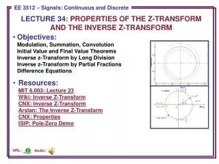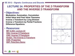
2. Z-transform and theorem
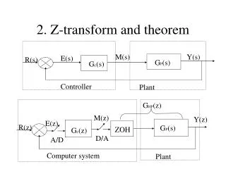
G HP (z). M(z). Y(z). M(s). Y(s). E(s). E(z). R(s). R(z). G P (s). G P (s). G c (s). ZOH. G c (z). D/A. A/D. Controller. Plant. Computer system. Plant. 2. Z-transform and theorem. f(kT). f(t). A/D . time. Time kT. f(kT). f(kT). D/A . Time kT. Time kT.

2. Z-transform and theorem
E N D
Presentation Transcript
GHP(z) M(z) Y(z) M(s) Y(s) E(s) E(z) R(s) R(z) GP(s) GP(s) Gc(s) ZOH Gc(z) D/A A/D Controller Plant Computer system Plant 2. Z-transform and theorem
f(kT) f(t) A/D time Time kT f(kT) f(kT) D/A Time kT Time kT 2. Z-transform and theorem
2. Z-transform and theorem How can we represent the sampled data mathematically? For continuous time system, we have a mathematical tool Laplace transform. It helps us to define the transfer function of a control system, analyse system stability and design a controller. Can we have a similar mathematical tool for discrete time system?
2.1 Z-transform For a continuous signal f(t), its sampled data can be written as, Then we can define Z-transform of f(t) as where z-1 represents one sampling period delay in time.
f(t) t f(kT) kT 2.1 Z-transform Solution: Example 1: Find the Z-transform of unit step function.
2.1 Z-transform Apply the definition of Z-transform, we have
2.1 Z-transform Another method
f(t) t 2.1 Z-transform Example 2: Find the Z-transform of a exponential decay. Solution:
f(t) t 2.1 Z-transform Exercise 1: Find the Z-transform of a exponential decay f(t)=e-at using other method.
2.1 Z-transform Example 3: Find the Z-transform of a cosine function. Solution: As
2.1 Z-transform Exercise 2: Find the Z-transform for decayed cosine function
2.1 Z-transform Example 4: Find the Z-transform for Solution:
2.1 Z-transform Exercise 3: Find the Z-transform for
2.1 Z-transform • The functions can be given either in time domain as f(t) or in S-domain as F(s). They are equivalent. eg. • A unit step function: 1(t) or 1/s • A ramp function: t or 1/s2 • f(t)=1-e-at or a/(s(s+a)) • etc.
2.2 Z-transform theorems Linearity: If f(t) and g(t) are Z-transformable and and are scalar, then the linear combination f(t)+g(t) has the Z-transform Z[f(t)+g(t)]= F(z)+ G(z)
f(t-nT) f(t) nT t t 2.2 Z-transform theorems Shifting Theorem: Given that the Z-transform of f(t) is F(z), find the Z-transform for f(t-nT).
2.2 Z-transform theorems If f(t)=0 for t<0 has the Z-transform F(z), then Proving: By Z-transform definition, we have
2.2 Z-transform theorems Defining m=k-n, we have Since f(mT)=0 for m<0, we can rewrite the above as Thus, if a function f(t) is delayed by nT, its Z-transform would be multiplied by z-n. Or, multiplication of a Z-transform by z-n has the effect of moving the function to the right by nT time. This is the so-called Shifting Theorem.
2.2 Z-transform theorems Final value theorem:Suppose that f(t), where f(t)=0 for t<0, has the Z-transform of F(z), then the final value of f(t) can be given by There are other theorems for Z-transform. Please read the study book or textbook for more details.
Theorem Name Definition Linearity Multiply by e-at Multiply by at Time Shift 1 Time Shift 2 Differentiation Integration Final Value Initial Value
f(t) F(s) F(z) (t) 1 1 u(t) t e-at 1 – e-at sint cost e-atsint e-atcost
2.3 Z-transform examples Example 1: Assume that f(k)=0 for k<0, find the Z-transform of f(k)=9k(2k-1)-2k+3, k=0,1,2…. Solution: Obvious f(k) is a combination of three sub-function 9k(2k-1), 2k and 3. Therefore, first we can apply linearity theorem to f(k). Second, sub-function 9k(2k-1) can be considered as a product of k and 2-12k, then we can apply the theorem of multiply by ak. Finally, we can find the answer by combining these three together.
f(t) 1 t 1 3 4 5 6 7 8 0 2 2.3 Z-transform examples Example 2: Obtain the Z-transform of the curve x(t) shown below.
2.3 Z-transform examples Solution: From the figure, we have K 0 1 2 3 4 5 6… f(k) 0 0 0 1/3 2/3 1 1… Apply the definition of Z-transform, we have
2.3 Z-transform examples Example 3: Find the Z-transform of Solution: Apply partial fraction to make F(s) as a sum of simpler terms.
2.4 Inverse Z-transform The inverse Z-transform: When F(z), the Z-transform of f(kT) or f(t), is given, the operation that determines the corresponding time sequence f(kT) is called as the Inverse Z-transform. We label inverse Z-transform as Z-1.
Z-transform = Inverse Z-transform 2.4 Inverse Z-transform
f(t) T 2T 3T 4T 5T 6T t 0 2.4 Inverse Z-transform The inverse Z-transform can yield the corresponding time sequence f(kt) uniquely. However, it says nothing about f(t). There might be numerous f(t) for a given f(kT).
f(t) x(kT) Zero-order Hold Low-pass Filter 2.4 Inverse Z-transform
2.5 Methods for Inverse Z-transform How can we find the time sequence for a given Z-transform? • Z-transform table Example 1: F(z)=1/(1-z-1), find f(kT). F(z)=1+z-1+z-2+z-3+… f(kT)=Z-1[F(z)]=1, for k=0, 1, 2, …
2.5 Inverse Z-transform examples Example 2: Given , Find f(kT). Solution: Apply partial-fraction-expansion to simplify F(z), then find the simpler terms from the Z-transform table. Then we need to determine k1 and k2
2.5 Inverse Z-transform examples Multiply (1-z-1) to both side and let z-1=1, we have
2.5 Inverse Z-transform examples Similar as the above, we let multiply (1-e-aTz-1) to both side and let z-1 =eaT, we have Finally, we have
2.5 Inverse Z-transform examples Exercise 4: Given the Z-transform Determine the initial and final values of f(kT), the inverse Z-transform of F(z), in a closed form. Hint: Partial-fraction-expansion, then use Z-transform table, and finally applying initial & final value theorems of Z-transform.
2.5 Inverse Z-transform examples 2) Direct division method Example 1:F(z)=1/(1+z-1), find f(kT).
2.5 Inverse Z-transform examples Finally, we obtain: F(z)=1-z-1+z-2-z-3+… K = 0 1 2 3 … F(kT)= 1 -1 1 -1 Example 2: Given , Find f(kT). Solution: Dividing the numerator by the denominator, we obtain
2.5 Inverse Z-transform examples Finally, we obtain: F(z)=1+ 4z-1 + 7z-2 + 10z-3+… K = 0 1 2 3 … F(kT)= 1 4 7 10… Exercise 5: , Find f(kT). Ans. :k 0 1 2 3 4 5… f(kT) 0 0.3679 0.8463 1 1 1…
2.5 Inverse Z-transform examples 3) Computational method using Matlab Example: Given find f(kT). Solution: num=[1 2 0]; den=[1 –2 1] Say we want the value of f(kT) for k=0 to 30 u=[1 zeros(1,30)]; F=filter(num, den, u) 1 4 7 10 13 16 19 22 25 28 31…
2.5 Inverse Z-transform examples Exercise 6: Given the Z-transform Use 1) the partial-fraction-expansion method and 2) the Matlab to find the inverse Z-transform of F(z). Answer: x(k)=-8.3333(0.5)k+8.333(0.8)k-2k(0.8)k-1 x(k)=0;0.5;0.05;–0.615;–1.2035;-1.6257;-1.8778…
Reading • Study book • Module 2: The Z-transform and theorems • Textbook • Chapter 2 : The Z-transform (pp23-50)
F() Krad/s -8 -4 4 8 Tutorial • Exercise: The frequency spectrum of a continuous-time signal is shown below. • What is the minimum sampling frequency for this signal to be sampled without aliasing. • If the above process were to be sampled at 10 Krad/s, sketch the resulting spectrum from –20 Krad/s to 20 Krad/s.
F() Krad/s -8 -4 4 8 Tutorial Solution: 1) From the spectrum, we can see that the bandwidth of the continuous signal is 8 Krad/s. The Sampling Theorem says that the sampling frequency must be at least twice the highest frequency component of the signal. Therefore, the minimum sampling frequency for this signal is 2*8=16 Krad/s.
F() -8 -4 2 4 6 8 10 12 14 16 18 Krad/s Tutorial 2) Spectrum of the sampled signal is formed by shifting up and down the spectrum of the original signal along the frequency axis at i times of sampling frequency. As s=10 Krad/s, for i =0, we have the figure in bold line. For i=1, we have the figure in bold-dot line.
F() -14 -8 -6 -4 -2 2 2 4 4 6 6 8 8 10 10 12 12 14 14 16 16 18 18 -18 Krad/s Krad/s Tutorial For I=-1, 2,… we have
f(t) t Tutorial Exercise 1: Find the Z-transform of a exponential decay f(t)=e-aT using other method.
Tutorial Exercise 2: Find the Z-transform for a decayed cosine function Solution 1: