Download
1 / 11
110 likes | 274 Vues
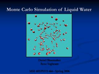
Monte Carlo Simulation of Liquid Water. Daniel Shoemaker Reza Toghraee MSE 485/PHYS 466 - Spring 2006. Objective. Write a MC liquid water simulation program from scratch which yields observables that are consistent with those found in the literature.

E N D
Monte Carlo Simulation of Liquid Water Daniel Shoemaker Reza Toghraee MSE 485/PHYS 466 - Spring 2006
Objective • Write a MC liquid water simulation program from scratch which yields observables that are consistent with those found in the literature. • We chose to code in C++ since it is modular and object-oriented. • The first decision we needed to make was which water potential to use.
Potentials • Many potentials exist for 2- 3- 4- and 5-site models of water. • We chose a 3-site NVT model to maintain simplicity while keeping good agreement with physical parameters. • TIP3P potential: • rOH = 0.96 Å • HOH angle = 104.52° • qO = -2qH = -0.834, charges located directly on atoms • LJA = 582x103 kcal Å12/mol, LJC = 595 kcal Å6/mol
Code Layout • Headers • Main.h • MC.h • Source • Main.cxx • Coordinates.cxx • Energy.cxx • GofR.cxx • MC.cxx • MCMove.cxx • RandGen.cxx • Necessary inputs: • Number of molecules • Temperature • Potential (TIP3P) • Initialization steps • MC steps • How often to sample Energy and g(r) • Volume calculated automatically from density • We used standard Intel and Microsoft math libraries and compilers.
Algorithm • Metropolis Monte Carlo algorithm: • Move random particle by a random distance • Calculate ∆E • Accept or reject move based on -1/kT • Update position • Our maximum movement length is 0.15Å to achieve an acceptance ratio between 43% and 64%, depending on the number of iterations. • Energy data is output every 1K-10K iterations, with g(r) data recorded about as often.
Optimization • Defining H positions without trig functions • Use linear algebra with properly generated random numbers to position the H atoms based on O • No lookup tables (trig functions) are used • Periodic Boundary Conditions • Setting up a 3x3x3 matrix of boxes that surround the core box is a quick way to find the shortest distance between to particles in PBC. • Much faster than subtracting nint(distance/box)*box from the distances
< Coulombic > = -0.918 +/- 0.015 < Lennard-Jones > = -1.53 +/- 0.12 < H binding > = -2.45 +/- 0.11 Iterations (x10) Energy Trends • Simulations were run with 10K initialization steps to ensure that the energy had settled. 3-D Potential Energies 2-D Hydrogen Binding Energy Iterations (x105)
Jorgensen et al Our Simulation Radial Distribution Function • g(r) does have a large initial peak, and a forbidden zone near r = 0, but its dimensions do not agree with theory
2-D Matlab Simulations • 2-D simulations show that water molecules cluster together. • In this simulation, all molecules are moved after every step.
Conclusions • Our program is a fast and intuitive way to simulate water using Monte Carlo. • This code can easily handle a 3-site potential, and minor modifications would allow 4-sites. • Our Lennard-Jones interactions are a little too strong, but the potentials behave as expected. • The g(r) normalization should be examined to correct its scale.
References • 2-D Simulations by Jihan Kim • Berendsen, H. J. C. et al, Intermolecular Forces, (D. Reidel Co., Holland 1983), 331. • Frenkel, D. and B. Smit, Understanding Molecular Simulation, (2nd Ed., Academic Press 2002). • Jorgensen, W. L., J. Am. Chem. Soc.103, 1981, 335. • Jorgensen, W. L. et al, J. Chem. Phys.79 (2), 12 July 1983, 926. • McDonald, I. R., Mol. Phys.23, 1972, 41.