Download
1 / 41
410 likes | 601 Vues
Estimating Heterogeneous Price Thresholds. Nobuhiko Terui* and Wirawan Dony Dahana Graduate School of Economics and Management Tohoku University Sendai 980-8576, Japan *E-mail:terui@econ.tohoku.ac.jp *Voice & Fax:+81-22-217-6311 International Conference at ISM.

E N D
Estimating Heterogeneous Price Thresholds Nobuhiko Terui*andWirawan Dony Dahana Graduate School of Economics and ManagementTohoku UniversitySendai 980-8576, Japan*E-mail:terui@econ.tohoku.ac.jp*Voice & Fax:+81-22-217-6311 International Conference at ISM
General nonlinear stochastic utility function :Domain of relevant threshold variable :Threshold points : Disjoint sub-domains
Nonlinear Random Utility Function- Asymmetric Market Response - 3 Regimes Model
Consumer Behavior Theory 1. Reference Price (RP) and its conceptualizations Adaptation-Level Theory 2. Asymmetric response around RP Prospect Theory 3. The Existence of Price Threshold Assimilation-Contrast Theory
The Object of This Research => Propose “Threshold Probit Model “in the form of incorporating these concepts together • Estimate Price Thresholds Latitude of Price Acceptance” at Household level. • Search for an Efficient Pricing through Customization Strategy
Tools ・Threshold Probit Model ・Hierarchical Bayes Modeling ・MCMC =>Gibbs Sampling for Response Parameters =>Metropolis-Hastings Sampling for Threshold Parameters
Threshold Probit Model and Hierarchical Bayes Modeling ●Choice Probability
●Likelihood for consumer h ●Total likelihood
●Between Subjects Model (1)Market Response (2)Price Threshold
●Price Threshold Models Note: Model 3 does not assume a priori insensitivity and it can be interpreted as price threshold model a posteriori when we observe the insignificant estimate of or in weaker form when the relation and is confirmed.
●HB(Hierarchical Bayes) Model (1)Heterogeneous parameter: (2)Homogeneous parameter: homogeneity Household “ h’ ” homogeneity
I.~V.=> Gibbs Sampling by Full Conditional Densities (Rossi, McCulloch and Allenby(1996)) VI. => Metropolis Sampling with Random Walk HB model for household h: Matrix notation: MCMC:
Empirical Results ●Marketing Mix Variables X = [Constant, Price, Display, Feature,Brand loyalty ] ( Display, Feature: 1 or 0) Price : log(price) Display and Feature: binary, Brand loyalty: smoothing variable over past purchases proposed by Guadagni and Little(1983) ●Reference Price ; Brand Specific RP (Breisch et al. (1997))
●Household Specific Variables = [Constant, Hsize, Expend, Pfreq] Hsize: 1-6(Number of Family), Expend: 9 categories (Shopping Expenditure / Month), Pfreq: 3 categories (Shopping Frequency), = [Constant, Hsize, Expend, Pfreq, Dprone, RP, BL] Dprone: deal proneness (Bucklin and Gupta(1992)) RP: reference price level (Kalyanaram and Little(1994)) BL: brand loyalty level (Kalyanaram and Little(1994)) ・Proportion of purchase (of any the five brands) made on promotion; ;
●LPA v.s. Household Characteristics “Expend” increases =>LPA is getting Wider “Hsize” increases => LPA is getting Narrower
●LPA v.s. Household Characteristics “Pfreq” increases => LPA is getting Wider “Dprone” increases => LPA is getting Narrower
●LPA v.s. Household Characteristics “BL” increases => LPA is getting Wider “RP” increases => LPA is getting Wider
●Marketing Mix Effectiveness ○ Price Gain (Regime 1) & Price Loss (Regime 3):: “Price” > “Display” > (”Brand Loyalty”) “Feature”, ○ LPA (Regime 2): “Display” > (”Brand Loyalty”>) “Feature”.
●Customized Pricing Figure 2: Expected Incremental Sales and Profits
[1] Customized Discounting I. α% discount from individual (lower) price threshold Conditional on (1)Expected Incremental Sales (Discount Promotion) (2)Expected Incremental Profit : (M: margin 0.3 assumption)
[2]Customized Price Hike Strategy II. α% price hike from individual (upper) price threshold Conditional on (1)Expected Incremental Sales (2)Expected Incremental Profit : (M: margin 0.3 assumption)
●Large Difference of Sales ・Between (LPA and LOSS) ・Between (LPA and GAIN)
●Maximal Profits happen at ・ r1h (Discounting) ・ r2h (Hike)
Non-customized Pricing (flat pricing) Manager does not now know the price thresholds => has to try possible levels f pricing. => d* = 0,±1, ±2, … , ±15% Compare their incremental profits with those of optimal customized pricing at r1h and r2h
[3] Difference from non-customized pricing (i) Discounting Conditional on depends on the regime determined by discount level Unconditional (ii) Price Hike
●Empirical Implications • A. Customized Discount Strategy (customized couponing) • Sales: • For every brand, there is a great difference of sales • increase between price gain regime and (negative) • LPA at • (2) The sales of most expensive brand E change most. • Profit: • Optimal discount levels happen at the lower price • threshold for every brand.
B. Customized Price Hike Strategy • Sales: • Large difference between inside and outside of the • upper price threshold for every brand. • Profit: • (2) The price hike at the level of makes • the incremental profits most.
Summary • Modeling • (i) Non-linear(piecewise linear) Random Utility • Price Threshold, • => Latitude of Price Acceptance • Asymmetric Market Response • (ii) Continuous Mixture Model (HB to Threshold Probit Model) • => Heterogeneous Consumers • (iii)
2.Empirical Findings and Implications (i) Price threshold models dominates Linear model =>Existence of Heterogeneous Price Threshold (ii) Marketing Mix Effectiveness ○ Price Gain &Loss Regimes: “Price” > “Display” > (”Brand Loyalty”) “Feature” ○ LPA Regime: “Display” > (”Brand Loyalty”) “Feature” (iii) Estimated “Heterogeneous Price Thresholds” => Incremental Profit r1h => Discounting(Target Couponing) r2h => Price Hike => Important information for customization strategy of pricing.