Model-Data Comparison of Mid-Continental Intensive Field Campaign Atmospheric CO 2 Mixing Ratios

1. Model-Data Comparison of Mid-Continental Intensive Field Campaign Atmospheric CO2 Mixing Ratios Liza I. Díaz May 10, 2010

2. Outline • Introduction • Mid-Continental Intensive Field Campaign • Motivation for this study • Methods • Results • Conclusion

3. Carbon Dioxide (CO2) • Understanding the CO2 balance is necessary because of the impacts this greenhouse gas has on the climate. • This motivated an interest to estimate the carbon budget. • Not all the CO2 emissions remain in the atmosphere; a portion of these emissions are taken up by the oceans and the terrestrial biosphere.

4. Sinks • Several studies concluded that a large net sink of CO2 must exist at temperate latitudes of the Northern Hemisphere (Tans et al., 1990; Ciais et al., 1995; Fan et al., 1998). Observations Models Tans et al., 1990

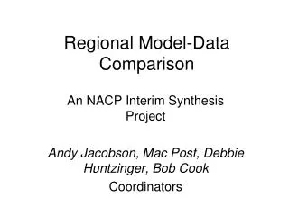
5. North American Carbon Program (NACP) • Goals include synthesizing models and observations, evaluating current modeling capability and investigating discrepancies between different flux estimates. • One method of estimating fluxes is the “top-down” or atmospheric inversion.

6. Atmospheric Inversions • Atmospheric inversions are highly variable. • This variability is caused by: • Lack of observations • Transport models NACP Interim Synthesis By : Andy Jacobson

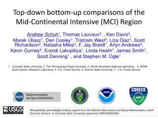
7. Mid-Continental Intensive (MCI) campaign • The main goal is to reach a convergence between the “top-down” atmospheric budget and agricultural inventory. • Tans et al.,(2005) proposed to study both approaches in a specific region and time so the information and credibility of each method could be maximized.

8. Mid-Continental Intensive (MCI) Region • MCI Region consists of: • Eastern South Dakota • Eastern Nebraska • Eastern Kansas • Northern Missouri • Iowa • Southern Minnesota • Southern Wisconsin • Illinois Main Reason  The agricultural production is recorded in detail which helps to provide accurate information on the carbon flux for the inventories.

9. Networks of CO2 measurements in the MCI Region • National Oceanic and Atmospheric Administration (NOAA) tall towers and trace gases sampling. • The Ring2 network managed by the Pennsylvania State University. • Location had the highest density of CO2 measurements to date. • A goal is to determine the density of measurements that is needed to understand the carbon budget.

10. Atmospheric Inversion • Temporal and spatial patterns in atmospheric CO2 mixing ratios are combined with a transport model to infer surface fluxes (Gurney et al., 2002; Rödenbeck et al., 2003; Baker et al., 2006).

11. Atmospheric Inversion Fluxes + Uncertainties Predicted [CO2] Obs. [CO2] Predicted [CO2] - Transport Model + Uncertainties

12. Atmospheric Inversion • The steps involved in an inverse model are: • Atmospheric CO2 concentrations are predicted by a forward model (a combination of a vegetation model with an atmospheric transport model). • Concentrations predicted by the forward model are compared to the observations. • Fluxes are adjusted to minimize the difference.

13. Objective • Evaluate the performance of a global atmospheric inversion in the MCI region. • Evaluate the statistical characteristics of the model-data differences needed to conduct an atmospheric inversion. • Examine atmospheric CO2 mixing ratio.

14. Methodology • Observations • PSU Ring of Towers • NOAA Tall Towers • Carbon Tracker Model • Transport Model (TM5) • Carnegie Ames Stanford Approach (CASA) • Data Selection • Statistics

15. Observation Location • Midwest agricultural belt in the northern U.S. • Distance between sites range from 125 to 370 km (Miles et al., to be submitted). • Three of these sites are located in the “corn belt”.

16. Ring2 • PSU Ring2 • Centerville, IA • Galesville, WI • Kewanee, IL • Mead, NE • Round Lake, MN • Sampling heights: 30 and 110-140 m AGL • In operation between April 2007 and November 2009

17. NOAA Tall Towers • NOAA Tall Towers • LEF, WI • Sampling heights: 11,30,76,122,244,396 m AGL • In operation: 1994-current • WBI, IA • Sampling heights: 31, 99, 379 m AGL • In operation: July 2007-current

18. Carbon Tracker Model • Calculates biogenic CO2 fluxes by integrating daily daytime average CO2 observations with an atmospheric transport model and a first guess of the biogenic fluxes. • Biogenic fluxes are optimized by minimizing the difference between observed and modeled atmospheric CO2.

19. Transport Model Version 5 (TM5) • Meteorological data is provided by the model of European Centre for Medium-Range Weather Forecast (ECMWF). • For this study TM5 is run at a horizontal resolution of 6°× 4° (longitude × latitude), with nested regions over: • North America (3°× 2°) • United States (1°× 1°) • Vertical resolution includes 25 vertical levels.

20. Carnegie Ames Stanford Approach (CASA) • Produces fluxes in a monthly time resolution and global 1°× 1° spatial resolution. • To calculate global fluxes CASA uses input from weather models and satellite- observed Normalized Difference Vegetation Index (NDVI).

21. Data Selection Daytime • Average mid-day CO2 observations 1800-2200 UTC. • Sampling levels of the observations around or above 100 m AGL. • Ignored nighttime data. Convective Boundary Layer

22. Choosing Model Level • First level of Carbon Tracker is approximately 200 to 400 m AGL but behaves like a surface layer. • Differences between levels 2,3 and 4 are less than 2 ppm. • Level 3 is used in Carbon Tracker assimilation system. • Therefore we use LEVEL 3.

23. Statistical Analysis • Two periods • June through December 2007 This period lets us evaluate the seasonal cycle over the year of 2007. • Growing Season 2007 (June through August) This period eliminates any seasonality and leaves day-to-day variability. During this season the variability of the mixing ratios are large because the fluxes are large.

24. Statistical Analysis • Time Series analysis • Model Performance • Taylor Diagram • Residual distributions • Gaussian fit • Temporal Correlations • Autocorrelations • Power Spectrum • Spatial Correlations • Relation between meteorological data and residuals

25. Time Series CO2 Observations • “Corn belt” sites with the highest drawdown. • Seasonal amplitude: • “corn belt” - 40 ppm • Sites with different vegetation – 24-29 ppm

26. Simulated and Observed Times Series Carbon Tracker Observation – Carbon Tracker • Carbon Tracker does not simulate these three “corn belt” sites drawdown correctly. • Possible causes to these differences: • Uptake is underestimated in the “corn belt” region. • Vertical mixing is too strong.

27. Statistical Analysis • Time Series analysis • Model Performance • Taylor Diagram • Residual distributions • Gaussian fit • Temporal Correlations • Autocorrelations • Power Spectrum • Spatial Correlations • Relation between meteorological data and residuals

28. June through December Taylor Diagram • Model is highly correlated with observations (R > 0.8). • The model underestimates the day-to-day variability for all the sites.

29. Growing Season Taylor Diagram • Model is less correlated with observations (R < 0.8),except Centerville site (R > 0.8). • The model underestimates the day-to-day variability for all the sites, except Centerville.

30. Taylor Diagram • Model can better simulate the seasonal cycle than synoptic variability. • Model tends to underestimate the amplitude of both the seasonal cycle and the day-to-day variability.

31. Statistical Analysis • Time Series analysis • Model Performance • Taylor Diagram • Residual distributions • Gaussian fit • Temporal Correlations • Autocorrelations • Power Spectrum • Spatial Correlations • Relation between meteorological data and residuals

32. June through December Distributions Galesville Round Lake • “Corn belt” sites have the highest standard deviation. • All of the sites are negatively skewed, except Centerville.

33. June through December Distributions

34. Growing Season Distribution Galesville Round Lake • In general “Corn belt” sites have the highest mean and standard deviation.

35. Growing Season Distribution

36. Gaussian Distribution June through December 2007 Growing Season 2007 • A χ2 test was performed to determine if distributions are Gaussian. • Limited number of samples make our χ2 inconsistent, but will be applied to hourly residuals.

37. Data Independence • Determine correlation in time: • Autocorrelations • Power Spectrum • Determine correlation in space: • Estimation of correlation across sites Motivation: Evaluate independence of the data in the inverse system.

38. Statistical Analysis • Time Series analysis • Model Performance • Taylor Diagram • Residual distributions • Gaussian fit • Temporal Correlations • Autocorrelations • Power Spectrum • Spatial Correlations • Relation between meteorological data and residuals

39. Temporal Correlation Centerville LEF • Centerville and LEF sites show the lowest correlation of residuals in time. • Centerville behaves completely different than the rest of the sites.

40. Temporal Correlation Round Lake WBI • Sites located in “corn belt” tend to show correlation of the residuals in time for a period of 40 to 50 days. • This autocorrelation shows an error in the seasonal cycle, because growing season lasts about 50 to 60 days in a year.

41. Statistical Analysis • Time Series analysis • Model Performance • Taylor Diagram • Residual distributions • Gaussian fit • Temporal Correlations • Autocorrelations • Power Spectrum • Spatial Correlations • Relation between meteorological data and residuals

42. Power Spectrum Round Lake WBI • This suggests that residuals have a maximum every 4 to 5 days for all the sites. • One possible cause for this is weather events. • Therefore, transport might be causing these changes in residuals.

43. Statistical Analysis • Time Series analysis • Model Performance • Taylor Diagram • Residual distributions • Gaussian fit • Temporal Correlations • Autocorrelations • Power Spectrum • Spatial Correlations • Relation between meteorological data and residuals

44. Spatial Correlation June through December 2007 • Two sites located at the “corn belt” are the highest correlated. • The second highest spatial correlation is WBI (corn belt) and Mead (mixed vegetation).

45. Spatial Correlation Growing Season 2007 • Two sites located at the “corn belt” are the highest correlated. • The second highest spatial correlation is Kewanee (corn belt) and Galesville (mixed vegetation).

46. Spatial Correlation • The only sites which residuals are highly correlated in space are WBI and Kewanee. • Both sites are part of the “corn belt” region. • However, spatial correlation of the residuals are weaker among the other “corn belt” sites. Distance: 125 km Vegetation: corn

47. Statistical Analysis • Time Series analysis • Model Performance • Taylor Diagram • Residual distributions • Gaussian fit • Temporal Correlations • Autocorrelations • Power Spectrum • Spatial Correlations • Relation between meteorological data and residuals

48. Wind Direction and Temperature June through December 2007 • Some of the sites like Round Lake shows a relationship between northerly winds and high residuals, but it is not clear. • High residuals are also correlated with high temperature. Basically this period is the growing season, in which not only are the temperatures high but also the fluxes are large.

49. Wind Direction and Temperature Growing Season 2007 • Centerville does not show any correlation between residuals and both temperature and wind direction. • Round Lake shows again weak relationship between high residuals and wind coming from the north. But, there is no correlation between temperature and residuals. • No persistent correlation between residuals and meteorological data.

50. Conclusions • Carbon Tracker does not well simulate “corn belt” draw down. • Carbon Tracker simulates better the seasonal cycle than it does the day-to-day variability. • Gaussian assumption might be violated and need to test what effect could cause in the inversion. • Residual differences or error are repeated through the growing season period. • Carbon Tracker shows a possible synoptic error. • Residuals show a weak spatial correlation amongst the sites, suggesting some independence of the error. • Residuals are not correlated to temperature, but some sites shows a weak correlation between residuals and wind coming from the North.