Download
1 / 46
460 likes | 741 Vues
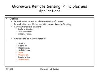
Microwave Remote Sensing of Atmospheric Trace Gases. Remote Sensing I Lecture 6 Summer 2006. J. F(J). Rotational Energy Levels. Rotational Transitions. allowed transitions:. Rotational Transitions. Microwave Spectrum of HCl. Microwave Spectrum of ClO. posible orientations.

E N D
Microwave Remote Sensing of Atmospheric Trace Gases Remote Sensing I Lecture 6 Summer 2006
J F(J) Rotational Energy Levels
allowed transitions: Rotational Transitions
posibleorientations Degeneracies of Rotations J=1
Degeneracies of Rotations J=2 J=3
Intensities of Rotational Lines • Probability for transition between level l and level udepends on the number of molecules in level l • In thermal equilibrium given by Boltzmann distribution: (tends to decrease with increasing J)
Intensities of Rotational Lines • Depends also on degenaracies of the levels: (tends to increase with increasing J) Overall proportional to:
Intensities of Rotational Lines May be used to derivetemperature from observedspectrum
The N2O Molecule N N O N2O is a linear molecule
The Water Molecule O 0.09578 nm 104.48° H H
Microwave Limb Sounding: MLS / UARS
Part 1: Airborne Microwave Remote Sensing of Atmospheric Trace Gases.
Part 2: Ground-based Microwave Remote Sensing of Atmospheric Trace Gases.
Pressure Broadening of Spectral Lines 50km / 0.5 hPa 20km / 50 hPa 10km / 200 hPa
Retrieval techniques / Inverse Modelling Assume that the measured spectrum y is a known function of the atmospheric profile x plus some noise ε. Linearize F (also known as the forward model):
Optimal Estimation However, can not be directly inverted (ill-posed problem) Best estimate given by Optimal Estimation solution: Best guess profile A-priori profile Measurement error covariance matrix A-priori profile covariance matrix
Optimal Estimation: Averaging Kernels Optimal estimation solution: Define: Then: Define Averaging Kernel MatrixA = DK: