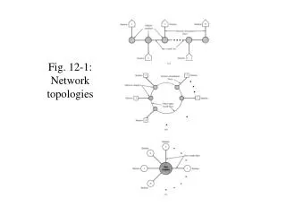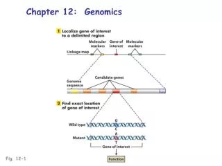
Fig. 12-1
430 likes | 696 Vues
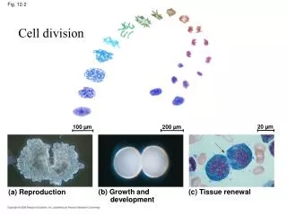
Chapter 12: Genomics. Fig. 12-1. Genomics: the study of whole-genome structure, organization, and function Structural genomics: the physical genome; whole genome mapping Functional genomics: the proteome, expression patterns, networks.

Fig. 12-1
E N D
Presentation Transcript
Chapter 12: Genomics Fig. 12-1
Genomics: the study of whole-genome structure, organization, and function Structural genomics: the physical genome; whole genome mapping Functional genomics: the proteome, expression patterns, networks
Creating a physical map of the genome • Create a comprehensive genomic library • (use a vector that incorporates huge fragments) • Order the clones by identifying overlapping groups • (e.g., sequencing ends to determine “contigs”) • Sequence each contig • Identify genes and chromosomal rearrangements • within each contig (correlates the genetic and • physical maps)
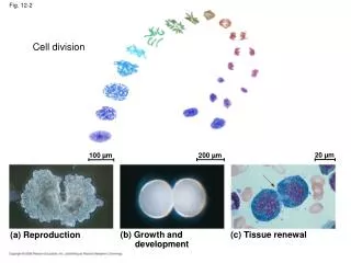
Overview of genome sequencing Fig. 12-2
Overview of genome sequencing Fig. 12-2
Overview of genome sequencing Fig. 12-3
Several orders of magnitude resolution separates cytogenetic from gene-level understanding Fig. 12-9
Creating a high-resolution genetic map • of the genome requires many “markers” • Classic mutations and allelic variations (too few) • Molecular polymorphisms; selectively neutral DNA • sequence variations are common in genomes • Example: Restriction Fragment Length Polymorphisms • (RFLP markers)
Inheritance of an RFLP: Fig. 12-10
Inheritance of an RFLP: Determining linkage to a known gene Fig. 12-10
Inheritance of an RFLP: Determining linkage to a known gene Fig. 12-10
Linkage analysis of a gene and VNTR markers Fig. 12-11
Creating a high-resolution genetic map • of the genome requires many “markers” • Classic mutations and allelic variations • Molecular polymorphisms; selectively neutral DNA • sequence variations are common in genomes • Example: Restriction Fragment Length Polymorphisms • (RFLP markers) • Example: Simple Sequence Length Polymorphisms • (SSLP markers)
SSLP: Simple sequence length • polymorphism • VNTR repeat clusters (minisatellite markers) • dinucleotide repeats (microsatellite markers) • VNTRs can be detected by restriction/Southern blot • analysis; both detected by PCR using primers for • each end of the repeat tract
Variable number tandem repeats (VNTRs) • “minisatellite” DNA • 15-100 bp units; repeated in 1-5 kb blocks • expansion/contraction of the block due to • meiotic unequal crossingover • crossingover so frequent that each individual • has unique pattern (revealed by genomic • Southern blot/hybridization analysis)
Using a SSLP marker to map a disease Fig. 12-12
Using a SSLP marker to map a disease Unlinked Linked to P Linked to p Unlinked Fig. 12-12
Polymorphism markers can provide a high resolution map Linkage map of human chromosome 1 Fig. 12-13
High-resolution cytogenetic mapping • is based on: • In situ hybridization: hybridization of known • sequences directly to chromosome preparations • Rearrangement break mapping • Radiation hybrid mapping
FISH analysis using a probe for a muscle protein gene Fig. 12-14
Survey clones from the region of the break to determine one that spans the break Fig. 12-16
Survey clones from the region of the break to determine one that spans the break FISH analysis locates the sequence and the breakpoint cytogenetically Fig. 12-16
Cytogenetic map of human chromosome 7 Fig. 12-24
Determining the sequence map sites of rearrangement breakpoints and other mutations Fig. 12-17
Mapping & determining a gene of interest Fig. 12-18
Genome sequencing projects • Sequence individual clones and subclones • (extensive use of robotics) • Identify overlaps to assemble sequence • contigs (extensive use of computer-assisted • analysis) • Identify putative genes by identifying open • reading frames, consensus sequences and • other bioinformatic tools
Once a genomic sequence is obtained, it is subjected to • bioinformatic analysis to determine structure and function • Identify apparent ORFs and consensus regulatory sequences • to identify potential genes • Identify corresponding cDNA (and EST) sequences to identify • genuine coding regions • Polypeptide similarity analysis (similarity to polypeptides • encoded in other genomes)
Genes and their components have characteristic sequences Bioinformatic analysis of raw sequences can suggest possible features Fig. 12-19
Confirmation of genes and their architecture is obtained by analysis of cDNAs cDNA subprojects are key facets of a genome project Fig. 12-20
High-resolution genomics arises through the combination of bioinformatics and experimentation Fig. 12-21
Using bioinformatics to make detailed gene predictions Fig. 12-22
Complete sequence and partial interpretation of a complete human chromosome Fig. 12-23
Comparative genomics reveals ancestral chromosome rearrangements Fig. 12-26
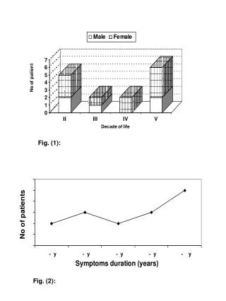
Microarray analysis – a form of functional genomics Arrays hybridized to cDNAs prepared from total RNA Relative intensity (color-coded) reflects abundance of individual RNAs 1046 cDNA array 65,000 oligo array (representing 1641 genes) Fig. 12-27