Chapter 13: Normal Distributions
This chapter focuses on exploring data for a single quantitative variable using normal distributions. Key techniques include creating histograms or stem-and-leaf plots to identify patterns and outliers. The chapter emphasizes quantifying data through five-number summaries, means, and standard deviations while employing density curves to describe data distribution. Important concepts like the empirical rule and standard scores are illustrated through real-world examples, including health data and standardized test scores. Understanding these distributions is crucial for accurate data interpretation and analysis.

Chapter 13: Normal Distributions
E N D
Presentation Transcript
Chapter 13: Normal Distributions Exploring data for one quantitative variable: • Always plot the data: Histogram or stemplot • Look for an overall pattern and for striking deviations such as outliers. • Describe center and spread with the five-number summary or the mean and standard deviation. • Overall pattern of a large number of observations is regular enough to be described by a smooth curve.
Density Curves Density curve: A curve that is superimposed on a density histogram to outline the shape. • The histogram shows the proportion in each class and the area under the curve is 1. • Density curves offer an easy and quick way of describing the shape of a distribution.
Using a Density Curve • Histograms show either frequencies (counts) or relative frequencies (proportions) in each class interval. • Density curves show the proportion of observations in any region by areas under the curve.
Center and Spread of a Density Curve Center: Three Measures • Mode: The most frequently occurring value(s). On a density curve, this is where highest point occurs. • Median: The point that divides the area under the curve in half. (p. 247) • Mean: The point at which the curve would balance if made out of solid material. (p. 247)
Symmetric and Skewed Curves • For a symmetric density curve, the mean, median, and mode are all equal. They lie in the center of the curve. • For a skewed density curve, the mean is pulled away from the mode and median in the direction of the long tail.
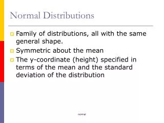
Normal Density Curves (p. 249) The normal curves are symmetric, bell-shaped curves that have these properties: • A specific normal curve is described by its mean and standard deviation. • The mean is the center of the distribution. It is located at the center of symmetry of the curve. • The standard deviation gives the shape of the curve. It is the distance from the mean to the change-of-curvature points on the other side.
Figure 13.7, p. 248: Mean and Standard Deviation For Two Normal Curves
Why Study Normal Curves? The normal curves are useful for describing many variables. Examples: • Health data: Heights, weight, blood pressure • Standardized test scores: SAT, GRE, IQ • Times in sporting events: Running, swimming, etc.
The “68-95-99.7 Rule” or The Empirical Rule (p. 250) In any normal distribution, approximately • 68% of the observations fall within one standard deviation of the mean. • 95% of the observations fall within two standard deviations of the mean. • 99.7% of the observations fall within three standard deviations of the mean
Example: IQ Scores for 12-year-olds IQ scores of 12-year-olds have normal distribution with a mean of 100 and a standard deviation of 16. • Compute an interval in which the middle 68% of scores will fall. Interval for 95%, 99.7%. • What percent of 12-year-olds will have IQ scores higher than 100? 116? 132? • What percent will have IQ scores lower than 116? 100? 84?
Standard Score (p. 252) • The standard score of an observation is the number of standard deviations away from the mean that the observation falls. • The standard score for any observation is Standard score = observation – mean standard deviation z= x -x s
Comparing Scores on SAT and ACT The SAT and the ACT measure the same kind of ability. • SAT verbal scores have a normal distribution with mean 500 and standard deviation 100. • ACT verbal scores are normally distributed with mean 18 and standard deviation 6. • Ricky scores 450 on the SAT and Seth scores 16 on the ACT. Who has the higher score? • Example 3 on p. 253: Similar example with two scores that are above the mean for each test.
Percentiles and the Normal Curve Percentiles: The cth percentile of a distribution is the value such that c percent of the observations lie below it and the rest of the observations lie above it. (p. 253) Table B, p. 547 gives standard scores and percentiles.
Percentiles on the SAT Example: Assume verbal SAT scores have an approximate normal distribution with a mean of 500 and a standard deviation of 100. • Suppose Fred receives a score of 400. What is Fred’s percentile rank? • Suppose Emma receives a score of 600. What is Emma’s percentile rank?