Propagation of Ultra-high Energy Cosmic Rays in Local Magnetic Fields

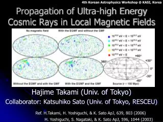
1. 4th Korean Astrophysics Workshop @ KASI, Korea Propagation of Ultra-high Energy Cosmic Rays in Local Magnetic Fields Hajime Takami (Univ. of Tokyo) Collaborator: Katsuhiko Sato (Univ. of Tokyo, RESCEU) Ref. H.Takami, H. Yoshiguchi, & K. Sato ApJ, 639, 803 (2006) H. Yoshiguchi, S. Nagataki, & K. Sato ApJ, 596, 1044 (2003)

2. Index 1. Introduction 2. Models of Magnetic Fields 3. Our Method for the UHECR Propagation 4. Results 5. Summary

3. Ultra-high Energy Cosmic Rays (UHECRs) UHECRs above 1019eV are highest energy cosmic rays. • Extragalactic origin ( larger than thickness of Galaxy ) • Light composition(?) • Expected to have small deflection angles in cosmic magnetic fields. • Expected to have the spectral cutoff due to photopion production with the CMB (GZK cutoff). ( Observed energy spectrum ) Whether there is the spectral cutoff or not is one of problems Auger and TA will solve this problem.

4. Arrival Distribution of UHECRs AGASA observation showed the arrival distribution is isotropic at large angle scale, but has strong correlation at small angle scale. Two Point correlation N(θ) E>4×1019eV 57 events(>1020eV 8 events) strong correlation at small angle （～ 3 deg） Isotropic at large angle scale However, HiRes observation showed the distribution has no small scale anisotropy. But this discrepancy between the two observations is not statistically significant at present observed event number (yoshiguchi et al. 2004).

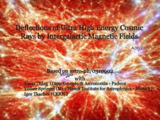
5. UHECR propagation in the Universe UHECRs experience energy losses and deflections due to cosmic magnetic field during the propagation in space. So the propagation processes are very important in order to simulate their arrival distribution and their energy spectrum at Earth. We consider • Energy loss processes (only in intergalactic space) • Interaction with the CMB • Pair creation ( Chodorowski et al. 1992 ) • Photopion production ( Mucke et al. 2000 ) • Adiabatic energy loss (due to the cosmic expansion) • Magnetic deflections • Due to extragalactic magnetic field (EGMF) • Due to Galactic magnetic field (GMF)

6. Our Study • We have performed numerical simulations of the propagation of UHECRs in a structured extragalactic magnetic field (EGMF) and Galactic magnetic field (GMF). • A new method for the calculation of the propagation in magnetic field is developed. • Our models of EGMF and distribution of UHECR sources reflect structures observed around the Milky Way. • We assume that UHECRs are protons above 1019eV. • The arrival distribution of UHECRs at the Earth is simulated and is compared with AGASA observation statistically. • From the comparison, we find number density of UHECR sources that reproduces the observation.

7. Index 1. Introduction 2. Models of Magnetic Fields 3. Our Method for the UHECR Propagation 4. Results 5. Summary

8. Observation of Magnetic Field Magnetic fields are little known theoretically and observationally. • EGMF There are observations of MFs from only clusters of galaxies. • The Faraday rotation measurement some evidence for the presence of MFs of a few uG ( Vogt et al. 2003 etc. ) • Hard X-ray emission average strength of intracluster MF within the emitting volume is 0.2-0.4 uG (Fusco-Femiano et al. 1999, Rephaeli et al. 1999) • GMF There are many observations with the Faraday rotation, of which most in Galactic plane. Models of magnetic fields should reflect these observational results. (Beck 2000)

9. Magnetic Fields expected by simulations Some groups have obtained local magnetic field by their cosmological simulations. Magnetic field generated from their simulation. They calculated the UHECR propagation. But observed local structures are not reproduced. Sigl et al. (2004) Matter density reproduces observed local structures. So Magnetic field is also thought to reproduce local structure. But they didn’t calculate the propagation. Dolag et al. (2005) We also construct EGMF model in order to calculate the propagation.

10. IRAS PSCz Catalog of galaxies We use the IRAS PSCz Catalog of galaxies to construct our structured EGMF model and models of sources of UHECRs. Large sky coverage Source model We select some of all the galaxies in this sample. The probability that a given galaxy is selected is proportional to its absolute luminosities. Only parameter is number density of galaxies.

11. Our structured EGMF model We assume density distribution from the IRAS catalog Strength of EGMF is normalized in the center of the Virgo cluster : 0.4 uG E=1019.6eV E=1020eV Deflection angles when CRs with fixed energies are propagated from the Earth to 100 Mpc. These figures show that our EGMF model reflects the distribution of the IRAS galaxies.

12. Model of Galactic Magnetic Field We adopt the same GMF model by Alvarez-Muniz et al. (2002) . dipole + spiral At the Solar system ～0.3uG ～1.5uG Top view of our Galaxy Top view of our Galaxy Side view of our Galaxy

13. Index 1. Introduction 2. Models of Magnetic Fields 3. Our Method for the UHECR Propagation 4. Results 5. Summary

14. A problem with the calculation If UHECR sources emit huge number of CRs, only very small fraction of CRs can reach the Earth due to magnetic deflections, but most of CRs cannot arrive at the Earth. This calculation takes a long CPU time to gather enough number of event at the Earth. Source Intergalactic Space (with EGMF) Our Galaxy Earth

15. A Solution of the Problem (1) Without EGMF, a method had been developed to solve the difficulty. ( Yoshiguchi et al., ApJ, 596, 1044 ) 1. CRs with a charge of -1 are ejected isotropically from the Earth 2. We then record their directions of velocities at ejection and r=40kpc (boundary between Galactic space and extragalactic space). 3. Finally, we select some of these trajectories so that the resulting mapping of velocity directions outside our galaxy corresponds to our source model. Galactic space 40kpc Earth G.C extragalactic space In this method, we can consider only UHECRs that reach the Earth.How can one calculate arrival distribution of UHE proton for a given source location scenario in detail ?

16. 2,000,000 “anti-protons” are ejected from Earth isotropically and their trajectories are recorded until 40 kpc. This map can be regarded as probability distribution for proton to be able to reach the earth in the case of isotropic source distribution. When we consider anisotropic source distribution, we multiply its effect to this probability distribution. one to one correspondence Arrival distribution of UHE protons at the earth is obtained.

17. A Solution of the Problem (2) Trajectories of CRs (Charge=-1) in Galactic space expand those in intergalactic space with EGMF. • The trajectories in intergalactic space are recorded. • When each trajectory passes galaxies (sources), the proton has a certain contribution to the “real”--- positive arriving--- CRs . • We regard the contribution factors of each CR as probabilities that the CR is a “real” event observed at Earth. • We select trajectories corresponding to the probabilities. Intergalactic Space (with EGMF) Source Our Galaxy Earth The arrival distribution ! This method gives us a natural expansion of our previous method. This method enables us to save the CPU time greatly.

18. Index 1. Introduction 2. Models of Magnetic Fields 3. Our Method for the UHECR Propagation 4. Results 5. Summary

19. Examples of trajectories in GMF Trajectories of “anti-protons” (E=1018.5eV) ejected from the earth in the direction b=0°(=protons arriving at Earth ) Only dipole field Only spiral field E=1018.5eV B Side view B Earth Top view The dipole field: exclude CRs from Galactic Center region. The spiral field: deflect CRs in the direction dependent on the direction of GMF near the Solar system.

20. Effect of GMF We can see the deflections about UHECRs above 1019eV. We eject cosmic rays above 1019eV with a charge of -1 from the Earth isotropically and follow them at 40 kpc from Galactic center. GMF Dipole field Spiral field Injection direction of CRs Velocity direction at 40kpc from GC Points in the right figure show source directions of them if extragalactic magnetic field is neglected.

21. An Arrival Distribution We simulate an arrival distribution in several conditions of MF. ns~10-5Mpc-3 UHECRs are arranged in the order of their energies, reflecting the directions of GMF. On the other hand, EGMF diffuse the arrival directions of UHECRs. The arrangement will allow us to obtain some kind of information about the composition of UHECRs and the GMF ( future works )

22. Two-point Correlation Functions 49 events ( 4×1019-1020eV ) • Histograms : observational result by AGASA. • Error bars : 1 sigma error due to finite event selections • Shade : 1 sigma total error including cosmic variance (source selection) ns~10-5Mpc-3 From comparison between panels, MFs, especially EGMF, makes the small-scale anisotropy be weaken. In many cases of source number density, we calculate the two-point correlation functions. The comparison to the observed results enables us to estimate source number density that best reproduces the observations.

23. Chi-square fitting with obs. data • Black : normal source model (NS) (power of each source independent of its luminosity ) • Red : luminosity weighted source model (LS) • Error bars : cosmic variance at fixed source number density The most appropreate source number density that reproduces the observation GMF + EGMF case No MF case NS model : ~10-5 Mpc-3 LS model : ~10-4 Mpc-3 NS model : ~10-6-10-5 Mpc-3 LS model : ~10-5-10-4 Mpc-3

24. Energy Spectrum GMF: Yes EGMF=0.0 uG EGMF=0.4 uG NS model@ 10-5 Mpc-3 Both cases reproduce observed spectra below 1020eV. UHECRs above 1020eV cannot be explained by our source model and are expected to have other origins. In the case of LS model, the same tendencies can be seen.

25. Index 1. Introduction 2. Models of Magnetic Fields 3. Our Method for the UHECR Propagation 4. Results 5. Summary

26. Summary • We performed numerical simulations of the propagation of UHECRs above 1019eV, considering a structured EGMF and GMF. • We developed a new method of simulations of the arrival distribution of UHECRs, applying to an inverse process, and simulated the distribution at Earth • Our EGMF model and source distribution that is constructed from the IRAS galaxies reflect the structures observed. • We estimate number density of UHECR source that best reproduces the AGASA observation. • Our source models reproduce observed spectra below 1020eV.