
Correspondences this week
Detailed analysis and results of performance comparison tests for C/C++ versus C# compilers on basic operations executed on Linux Ubuntu and Windows 7 systems.

Correspondences this week
E N D
Presentation Transcript
Correspondences this week From: Arjun Roy Sent: Sunday, March 02, 2014 8:14 PM Subject: C++/C# Compiler I did some tests to compare C/C++ Vs C# on some basic operation to see if the compilers handle the cases differently. I executed Dr. Wettstein's code in libPree library on Linux Ubuntu 12.04 and my C# code on Windows 7. 4 GB RAM. C/C++ C# OR 1 million 1.1 sec 0.1013 millisec OR 10 million 23.33 sec 1.016 millisec OR 100 million 266.38 sec 10.4494 millisec AND 1 million 0.99 sec 0.0989 millisec AND 10 million 23.29 sec 1.0235 millisec AND 100 million 279.92 sec 10.6166 millisec Number of 1's 1 million 0.49 sec 0.9647 millisec Number of 1's 10 million 5.11 sec 6.6821 millisec Number of 1's 100 million 55.73 sec 57.8274 millisec Either I am doing something incredibly wrong or these results are just great from C# point of view. Md, please run some test with Dr. Wettstein's code? I can ask Damien in the middle of the week about C# timings. Thanks,Arjun From: Mark Sent: March 03, 2014 To: William; Damian Subject: n-sphere density... In preparation for coding the faust cluster, I looked at the density calculation. As we are dealing with highly dimensional data, I looked at an approx of n-ball volume – it looks like this value falls very quickly to 0 as the number of dims increase, which makes this a bit hard to use…. My first thought was that we don’t really care that we don’t have a precise measurement of density since this is really just a knob someone is turning, and they will stop when they see meaningful clusters. However, the knob should behave the same way if we have 10,000 dimensions as it does if we have 3, and I suspect it does matter. Thoughts? From: William Sent: March 03, 2014 To: 'Mark... 1. Count of objects in the n=sphere may also fall quickly to zero, If it falls at about the same rate as volume, then density (quotient of them) should remain meaningful for large n 2. Theorem limitninfinityvolume(nsphere(r))=0 is true for all radii, r, but convergence is slower the higher the r. The n at which the volume peaks gets high for large r. There's a formula for that peak dim (as a function of r) but it's nasty. Might be a simpler calc giving us an r that pushes the peak out near the dataset dimension(e.g., n=10,000). That r would still give us a density but not a local one (getting a very average density measure rather than a precise local one). 3. Attribute elimination thru relevance analysis may be required in order to get a meaningful clustering (reducing n). The question is “Relevant to what?” since there is no class label. That’s why we’ve looked into variance measurements. They provide some basis for eliminating columns – if a column has low variance, it may not contribute to big gaps… I’m hoping 1. Is solution, but will continue to look into it this week. From: William Sent: Tuesday, March 04, 2014 9:24 AM To: 'Mark; 'Damian' So for the calculation, do we just get radius from the furthest point to the mean, count points in the cluster, and divide by n-ball volume? Should work, but requires the following steps (expensive?): 1. Calculate the SPTS, SQDM = (X-Mean) dot (X-Mean) 2. Approximate the maximum value in the SPTS, SQDM. We don’t need to identify furthest point. We just need the approx distance to it, by: IF OneCount{ HiBit(SQDM) & 2ndHiBit(SQDM) } >0 r ~= 2^(HiBit)+2*(2ndHiBit). ELSE r ~= 2^(HiBit) (where HiBit is the highest bit of SQDM with Count > 0) Building SQDM is expensive, so it might work just as well to do the above thing to a SPTS that we get for free, namely the column of the given X with maximum RawSpread=Max-Min (Outlier elimination may not be necessary – it gives a “CoreSpread” measurement): Let Xk be column with maximum [core] spread (maximizes (max-min) after outliers are removed from both ends leaving core of the Xk values). CoreSpread(Xk) / 2 should be a fairly good approx. of radius. Calculate CoreSpread(Xi) for i=1..n Set r = Median[CoreSpread(Xi)] / 2 (to guard against r being taken too large by virtue of one terribly elongated dimension.) From Mark: How about a quick and dirty to calculate candidates, aka hob dist between max and min - fast? I gather we don't need to be exact. we just want a suitable candidate.
FAUST Clusterers, 03/01/2014 A Clusterer (an unsupervised analytic) analyzes data objects without consulting a known class label (usually none are present). Objects are clustered (grouped) using a mechanism which attempts to maximize intra-classsimilarity and minimize inter-classsimilarity. Clustering facilitates taxonomy formation (organizing objects into a hierarchy that group similar events together (what a dendogram does?). FAUST Count Change clusterer FCC clusterer 1.Choose next D plan to use upon recursing, e.g., always AM, AFFA, FFAFFF, cycle thru e1..en,e1e2.., AM, AFFA, FFAFFF.. Choose a DensityThreshold (DT), DensityUniformityThreshold(DUT), PrecipitousCountChangeThreshold(PCCT). 2. If DT or DUT are not exceeded at a dendogram node (a cluster), partition that node as follows: 2a. Apply UDR (hi-to-lo bitslice) until a PCC appears, then build UDR branch down to a PCC pt or until PCC disappears. 2b. Cut at each singleton PCC. FCC cluster Notes: As will be obvious from the next slide, deciding on and using PCCT is a challenge. Expensive parts? Creating some of the SPTSs, e.g., XoD for D other than a diagonal. Finding PCC using UDR FAUST Anomaly Detector, FAD(outlier detection analytic) identify objects not complying with data model. Outliers are discarded as noise or exceptions, but in some applications, e.g., fraud detection, rare events are more interesting. Outliers detected with Statistics, Distance, Density and Deviation (use a dissimilarity measure to reduce overall dissimilarity by removing "deviation outliers") outlier detectors. Statistical tests assume a distribution/probability model, Outlier mining can mean: 1. Given a set of n objects and k, find the top k objects in terms of dissimilarity from the rest of the objects. 2. Given a Training Set, identify outlier objects within each class (correctly classified but noticeably dissimilar. 3. Determine "fuzzy" clusters, i.e., assign a weight for each object in each cluster (Does a dendogram do that?). We believe that FAUST Count Change clusterer is the best Anomaly Detector we have at this time.
FCC on IRIS150DT=1 PCCs have to involve a high of at least 5 and be at least 60% change from high. Gaps must be at least 3 60 62 63 64 65 66 67 69 71 72 73 75 76 78 79 83 88 2 1 1 4 2 3 3 2 4 3 1 3 2 1 2 2 1 2 1 1 1 1 1 2 2 1 1 2 1 2 1 4 5 64 65 67 68 69 70 71 72 73 74 75 77 78 80 81 82 83 84 85 86 89 96 98 3 2 3 1 1 2 2 2 3 3 1 1 3 2 1 4 1 1 1 2 1 1 1 1 2 1 1 1 1 1 1 1 1 2 1 2 1 1 1 1 1 1 3 7 2 5 F 0 3 6 7 8 9 10 11 12 13 14 15 16 17 18 19 21 22 23 26 27 28 Ct 1 1 3 2 6 4 2 3 5 4 2 4 2 4 2 2 1 1 1 1 3 1 GP 3 3 1 1 1 1 1 1 1 1 1 1 1 1 1 2 1 1 3 1 1 4 F 0 10 12 13 14 15 16 17 18 20 22 23 24 25 26 27 29 30 31 32 33 34 Ct 1 1 1 2 1 1 5 3 2 2 2 5 3 4 3 2 4 1 1 4 2 2 GP 10 2 1 1 1 1 1 1 2 2 1 1 1 1 1 2 1 1 1 1 1 1 35 36 37 38 41 42 43 45 46 47 48 50 51 52 53 55 56 57 58 59 60 62 63 2 1 3 2 2 2 2 3 1 3 1 1 1 6 1 3 3 2 5 2 3 4 2 1 1 1 3 1 1 2 1 1 1 2 1 1 1 2 1 1 1 1 1 2 1 1 103 1 32 33 34 36 37 39 41 42 43 45 46 47 48 49 50 51 53 54 55 56 57 58 59 2 1 1 1 1 5 2 1 4 3 2 1 4 2 4 5 1 2 5 3 2 5 1 1 1 2 1 2 2 1 1 2 1 1 1 1 1 1 2 1 1 1 1 1 1 1 Gap Preservation: Let Dk = ekoX + j<kmax(eioX) and use the SPTS, S= k=1..nDk (the idea is to make sure that gaps and PCCs in one dimension do not cancel out those of another dimension. If Card(X)=1,000,000,000,000, then Card(S) could be n times that large. However, the number of bitslices (pTrees) goes from log2(1,000,000,000,000) ~= 40 up by only a factor of log2n. I f n=1,000,000, then log2n ~= 20 so the number of pTrees increases from 40 to 60. Or can we accomplish the same thing by just shifting column values as follows: If D=(D1,D2,D3,D4) then let Y1=X1- minD1oX1 Y2=X2+maxD2oY1 Y3=X3+maxD3oY2 Y4=X4+maxD4oY3 Also, is there a better measure of gap potential than STD? How about St Std(Xk-minXk)/SpreadXk ? St1 St2 St3 St4 .22 .18 .29 .31 Using the above Gap Preservation method with D=1111 C2 (6s,0e,0i) C3 (14s,0e,0i) C4 (28s,10e,1i) C5 (1s,13e,2i) C6 (0s,6e,0i) C7 (0s,8e,1i) C8 (0s,4e,1i) C1 (1s,0e,0i) 85% accurate on 1st round! C10 (0s,0e,4i) C9 (0s,9e,41i) Using the Gap Preservation method with D=1011 C6 (0s,26e,2i) C3 (0s,4e,1i) C4 (0s,6e,0i) C5 (0s,5e,0i) C7 (0s,3e,0i) C8 (0s,4e,6i) C9 (0s,1e,4i) C1 | (6s,0e,0i) | C2 (43s,0e,0i) 94% accurate on 1st round! So the suggested best algorithm is : C11 (0s,0e,3i) C10 (0s,34e,1i) Set Dk to 1 for each column with St>ThrSt (Here ThrSt=0.2, so D=1011). Make Gap and PCC cuts on YoD, where Y is Gap Preserving shift of X
FCC on IRIS 1st 10 of each class= TestSet For a change to be Precipitous, it must be > 8 (which is 8/120=.067 of the TrainingSet) [0,64) 120 [0,32) 118 [32,64) 2(Drop this branch) 1 =25 bit 0 0 1 =24 bit [0,16) 68 [16,32) 50 [32,48) [48,64) 1 =23 bit 0 0 1 [0,8) 15 [8,16) 53 [16,24) 44 [24,32) 6(Drop branch) 1 =22 bit 0 0 0 1 1 [0,4)3[4,8)12 [8,12)21 [12,16)32 [16,20)28 [20,24)16 =21 bit 1 0 1 1 0 1 0 1 0 0 [4,6)4 [6,8)8 [8,10)9 [10,12)12 [12,14)19 [14,16)13 [16,18)12 [18,20)16 [20,22)11 [22,24)5 1 =20 bit 1 1 1 1 1 1 0 0 0 0 0 0 1 0 84 95 107 115 128 1311 146 157 168 174 1810 196 204 217 Should PCCT be reduced as you go down tree? Yes, since absolute change starts small and builds in round cluster Avg 50.4 34.4 14.6 2.5 Med 51 35 15 2 D=AM 0.57 0.55 0.32 -0.5 So then at 20 level, we might use PCCT=4, so we would cut at 13.5 and 17.5 Having checked, these cutpoints are not so good F < 13.5: s=34, e=14, i= 4 13.5 < F < 17.5: s= 5, e=15, i= 7 17.5 < F s= 1, e=11, i=29 The reason may be Avg and Med are so close (which will be the case for most larger datasets). I will try ek and other diagonals. 0 1 0 1 2 3 0 1 2 3 4 5 6 7 0 1 2 3 4 5 6 7 8 9 0 1 2 3 4 5 1 0 1 2 3 4 5 6 7 8 9 0 1 2 3 4 5 6 7 8 9 0 1 2 3 4 5 6 7 8 9 0 1 1 2 3 0 1 2 3 4 5 6 7 8 9 0 1 2 3 4 5 6 7 8 9 0 1 2 3 4 5 6 7 8 9 0 1 2 3 4 5 6 7 8 9 0 1 2 3 4 5 6 7 8 9 0 1 2 3 4 5 6 7 8 9 0 1 2 3 1 2 3 4 5 6
FCC on IRIS150 STDs: 8 4 17 7 Ordering: e3 e1 e4 e2 (The layout is: (CountsBetweenCutPoints) DensityBetweenCutPointsXoD_CutPoint ) Density Count / (AvgSpread/2)2 OverallDensityIRIS150=ODI=0.47 Set DT at ~2 times ODI, DT=1 Why 2 times? Just a guess! 5 2 5 13 8 12 4 2 10 On C4 D=e4 dist: 9 10 11 12 13 14 15 16 17 So cut at PCCs 10, 16 On C4,2 D=e3 Cut at PCCs 47, 49 (0s,7e,0i) [0.8]10.5` (0s,38e,4i)[0.9]16(0s,2e,10i)[0.4] (0s,7e,0i) [0.8]47` (0s,3e,0i)[0.9]49(0s,2e,10i)[0.4] C4,1 C4,2 C4,3 C4,2,1 C4,2,2 C4,2,3 On C1, e1 ct 15 (50s,0e,0i) [1.3]15(0s,0e,1i)[] C1,1 C1,2 On X with D=e3=(0,0,1,0) (50s,0e,1i) [0.97] 14` (0s,1e,0i)[]21(0s,2e,0i)[32]24(0s,47e,43i)[0.8] 52 (0s,0e,1i)[]55(0s,0e,1i)[]58(0s,0e,1i)[] C1 C2 C3C4 C5 C6 C7
FCC on IRIS120 For a change to be Precipitous, it must be > 8 (which is 8/120=.067 of the TrainingSet) Density Count / (AvgSpread/2)2 OverallDensityIRIS120=ODI= .375 Set DT at approx 3 times ODI, DT=1. Why 3 times? Just a guess! 3 1 2 1 3 6 4 7 2 3 2 C4 e2 ctpts 4,13 2 3 4 5 6 7 8 9 10 11 12 13 14 C42, e3 ctpts 19 34 44 34 (0s,7e,10i) [1.1]44` (0s,0e,3i)[1.1] (0s,0e,1i) []19` (0s,4e,0i)[1.8] (0s,3e,1i) [.71]4` (0s,11e,16i)[.24]13(0s,1e,2i)[.4] C4,1 C4,2 C4,3 C4,2,1 C4,2,2 C4,2,3 C4,2,4 2 3 3 4 3 2 4 2 1 2 1 1 1 1 1 On C3, the e2=(0100) cutpoints are 12, 16, 21 Distribution:4 5 6 7 8 9 10 11 12 13 14 15 16 17 18 19 20 21 22 23 24 C4,3,1 e4 ctpt 11.5 (0s, 17e, 4i) [.88]12` (3s, 0e, 0i)[3]16(5s, 0e ,0i)[1.4]21(2s, 0e, 0i)[2.6] (0s,2e,6i) [.8]11.5` (0s, 1e, 2i)[.8] C4,3 e3 cpt 11.5 C41, e3 ctpt 38 C4,3,1,1 C4,3,1,2 (0s,2e,6i) [.8]11.5` (0s, 1e, 2i)[.8] (0s,3e,0i) [1]38` (0s, 0e, 1i)[] C4,3,1 C4,3,2 C4,1,1 C4,1,2 2 1 1 1 1 1 1 1 1 4 5 2 2 C5, e2=(0100) ctpts 9gp 11.5PCD Dis 8 9 10 11 12 13 C5,2, e3 ctpts 35.5 38.5 43 dist: 34 35 36 37 38 39 40 41 42 43 44 45 46 (0s,2e,0i) [32]35.5` (0s, 1e, 0i)[]38.5(0s, 1e, 2i)[1.6]43(0s,0e,3i)[3] (0s,1e,0i) []9` (0s,4e,5i)[0.85]11.5(0s,0e 4i)[3.2] C5,1 C5,2 C5,3 C5,2,1 C5,2,2 C5,2,3 C5,2,4 The UDR tree, using D=e1=(1,0,0,0): 2^5: 115 5 2^4: 66 51 5 2^3: 22 42 35 16 5 2^2: 6 16 17 25 19 16 13 3 4 1 2^1: 3 3 6 2 10 11 12 13 9 10 12 4 10 3 2 1 0 4 1 2^0: 1 2 1 2 1 5 2 8 8 3 1 5 6 6 7 6 3 6 6 4 6 6 3 1 7 3 3 0 0 2 0 1 0 0 4 0 1 0 1 2 3 4 5 6 7 8 9 0 1 2 3 4 5 6 7 8 9 0 1 2 3 4 5 6 7 8 9 0 1 2 3 4 5 6 7 8 9 0 1 2 3 4 5 6 7 8 9 0 1 2 3 4 5 6 7 8 9 0 1 2 3 1 2 3 4 5 6 On X, the e1=(1,0,0,0) cutpoints are 6,10,16,23,28,33 (layout is: (ClassCountsBetweenCutPoints) DensityBetweenCutPointsXod_CutPoint ) (12s,0e,0i) [1.6]6` (18s,3e,0i)[.4]10(10s,17e,4i)[.3]16(0s,15e,19i)[.4]23 (0s,5e,9i)[.8]28(0s,0e,3i)[1.3]33(0s,0e,5i)[.5] C1 C2 C3 C4 C5 C6 C7 On C2, the e2=(0,1,0,0) cutpoints are 7.5, 16, 19.5 (0s, 3e, 0i) [1.3]7.5` (13s, 0e, 0i)[2,6]16(4s, 10e, 0i)[5.2]19.5(1s, 0e, 0i)[64] C2,1 C2,2 C2,3 C2,4 C3,1 C3,2 C3,3 C3,4 0 1 0 1 2 3 0 1 2 3 4 5 6 7 0 1 2 3 4 5 6 7 8 9 0 1 2 3 4 5 1 0 1 2 3 4 5 6 7 8 9 0 1 2 3 4 5 6 7 8 9 0 1 2 3 4 5 6 7 8 9 0 1 1 2 3 0 1 2 3 4 5 6 7 8 9 0 1 2 3 4 5 6 7 8 9 0 1 2 3 4 5 6 7 8 9 0 1 2 3 4 5 6 7 8 9 0 1 2 3 4 5 6 7 8 9 0 1 2 3 4 5 6 7 8 9 0 1 2 3 1 2 3 4 5 6
FCC on IRIS150 diagonals will be ordering by std(Layout: (CountsBetweenCutPoints) DensityBetweenCutPointsXoD_CutPoint ) Set DT=1 std diag 17.6 3 12.5 1+3 12.4 3+4 10.7 1+3+4 9.91 2-3 9.00 2-3-4 8.95 1-2+3 8.51 1-2+3+4 8.25 1 8.15 2+3 8.01 1+2+3 7.85 2+3+4 7.79 1+2+3+4 7.60 4 7.56 1+4 6.11 1-3-4 6.06 1+3-4 5.62 1-3 5.33 3-4 5.21 1+2-3-4 F 0 1 2 3 4 5 6 7 8 9 20 23 25 26 27 28 29 30 31 32 33 34 35 Ct 1 1 2 7 12 14 7 4 1 2 1 2 2 1 1 1 3 5 3 4 2 4 8 Gp 1 1 1 1 1 1 1 1 1 11 3 2 1 1 1 1 1 1 1 1 1 1 1 36 37 38 39 40 41 42 43 44 45 46 47 48 49 50 51 53 54 56 57 59 3 5 3 5 4 8 2 2 2 3 6 3 3 2 2 3 1 1 1 2 1 1 1 1 1 1 1 1 1 1 1 1 1 1 1 1 2 1 2 1 2 On C4 with D=e1=(1,0,0,0) F 13 14 15 16 17 18 19 20 22 23 24 25 26 27 Ct 1 1 3 2 2 4 1 5 2 1 2 1 2 1 Gp 1 1 1 1 1 1 1 2 1 1 1 1 1 gap1 gap2 pcc1 pcc2 On X with D=e3=(0,0,1,0) 0(50s,0e,1i)[2.5]15 C1 15(0s,3e,0i)[1.3]24 C2 24 (0s,33e,1i)[1.3]35.5 C3 35.5 (0s,14e,14i)[.3]41.5 C4 41.5 (0s,0e,34i)[1.3]99 C5 pcc2 pcc3 pcc4 pcc5 pcc1 17.5(0s,3e,1i)[.5]18.5 C4,3 19.5(0s,2e,3i)[.2]20.5 C4,5 18.5(0s,0e,1i)[]19.5 C4,4 20.5(0s,7e,2i)[.2]99 C4,6 14.5(0s,2e,5i)[.5]17.5 C4,2 0(0s,0e,2i)[2.5]14.5 C4,1
FCC on IRIS150DT=1 PCCs have to involve a high of at least 5 and be at least 60% change from high. Gaps must be at least 3 F 0 3 4 5 6 7 8 9 10 11 12 13 14 15 16 17 18 19 20 21 22 37 Ct 1 1 2 1 1 2 3 1 6 5 2 5 4 4 3 2 3 1 1 1 1 2 Gp 3 1 1 1 1 1 1 1 1 1 1 1 1 1 1 1 1 1 1 1 15 1 38 40 41 47 49 50 51 53 54 55 56 57 59 60 61 63 65 66 67 69 70 71 72 73 1 1 1 2 1 2 1 2 2 3 5 1 2 1 2 1 4 2 2 2 5 2 3 5 2 1 6 2 1 1 2 1 1 1 1 2 1 1 2 2 1 1 2 1 1 1 1 1 F 74 75 76 77 78 79 81 82 83 84 85 86 87 88 89 90 91 92 93 94 95 96 99 Ct 2 2 2 1 2 1 2 3 1 1 1 1 2 3 2 2 1 1 1 2 2 1 2 Gp 1 1 1 1 1 2 1 1 1 1 1 1 1 1 1 1 1 1 1 1 1 3 4 103 106 108 109 111 114 1 1 2 1 1 1 3 2 1 2 3 On X with D=1+3+4=(1,0,1,1) C1 (1s,0e,0i) C2 (11s,0e,0i) C3 (11s,0e,0i) C4 (2s,0e,0i) C5 (25s,0e,0i) C6 (0s,4e,0i) C7 (0s,0e,1i) C8 (0s,17e,1i) C9 (0s,17e,0i) C10 (0s,3e,2i) C11 (0s,4e,6i) 93.3% accurate on 1st round! C12 (0s,5e,31i) C13 (0s,0e,2i) C14 (0s,0e,1i) C15 (0s,0e,5i) C16 (0s,0e,1i) 2nd dendogram level: On C12 I had to cheat (Use D=(.28 .03 -.7 -.6) which connects class means. This does tell us: There is a vector which does it, but not how to find it?) On C11 D=e2= (0100) F 5 7 8 10 13 Ct 2 3 2 2 1 Gp 2 1 2 3 F 2 5 6 7 8 9 10 11 12 14 15 18 20 Ct 1 4 1 7 3 2 5 4 2 2 1 3 1 Gp 3 1 1 1 1 1 1 1 2 1 3 2 C11,1 (0s,1e,1i) C11,4 (0s,1e,0i) C11,2 (0s,2e,3i) C11,3 (0s,0e,2i) C12,2 (0s,1e,4i) C12,3 (0s,0e,1i) C12,1 (0s,0e,5i) On C8 D=e2= (0100) doesn't separate. So (w/o the cheat) 95% accurate after 2nd round! On C10 D=e2= (0100) F 2 8 9 11 12 Ct 1 1 1 1 1 Gp 6 1 2 1 C10,2 (0s,0e,3i) C10,3 (0s,2e,0i) C10,1 (0s,0e,1i) STD(F) DIAGONAL 34. 1+3+4 32. 1-2+3+4 31. 1+2+3+4 27. 2-3-4 26. 1-2+3 25. 1+3 24. 3+4 24. 1+2+3 23. 2+3+4 20. 1+2-3-4 19. 1-2+3-4 19. 2-3 18. 1-3-4 18. 1+3-4 17. 3
FAUST Classifiers, 03/2014 FAUST Spherical Classifier: y isa Ck iff OneCount{Ck-y)o(Ck-y) rk2} is the maximum over k=1..K FAUST Linear ClassifierConstruct hull, Hk, about Ckx isa Ck iff xHk. (allows "none of the above" when xHk, k.) Hks parallel constr Classifier(supervised analytic) constructs a model that distinguish classes, then use it to predict the class of unclassified objects. Models are constructed from a training set (table of objects with class labels). Classification may need to be preceded by relevance analysis to eliminate attributes that do not seem to contribute much information as to class. Summary of FAUST Classifiers: X=(X1..Xn,C)=TrainingSet (classified objects) Y=(Y1..Yn)=TestSet (unclassified objects) Classes: C1..CK FAUST Centroid Classifier: Separate classes, Ci and Cj, with a CutPoint, ci,j, in the SPTS, XoDi,j, with D being the vector: Di,jMeanCiMeanCj (or use VectorsOfMedians) ci,j=MdPt(D) (or use VarianceRatios) y isa Ck iff yoDk,j<ck,j k SPTS primitives: Assume ClassMeans (VoMs) have been precomputed! Need only the (n2-n)/2 SPTSs, YoDk,j (concurrent) Advantages: Very fast. Extendable to a fuzzy classifier: weightCi(y) = ji| ci,j - yoDi,j| ???? Disadvantages: For none of the above, need a separate step: yCk, check d2(y,Ck)=(y-Ck)o(y-Ck)? (very expensive!) SPTS primitives: (Ck-y)o(Ck-y) SPTS is needed (y, k) pair, where yY and k=1..n Advantages: Full 1-class w none of the above. Extendable to fuzzy classifier: wtCi(y) = OneCount{(Ci-y)o(Ci-y)ri2} Disadvantages: Classifies one y at a time. Hard to decide on the values of (r1,...rn)? Slow! For each in a series of vectors, D, let loD,kmnCkoD (or the 1st PCI); hiD,kmxCkoD (or the last PCD). Classify yCk iff loD,k Doy hiD,k D. SPTS primitives: Compute CkoD k=1..n,D 1 time. Min, Max of SPTSs. D,y need Doy (form Y into a PTS, DoY, D?) Advantages: Full 1-class w none of the above. fast! Fuzzy extension: wt(y,k)=dis(y to Hk bddry)? Bulk classification Disadvantages: Hard to decide on the value of l and h? Accuracy may suffer a bit. Reduce the PCCT as you go down the tree? (as we enter a round cluster, the absolute change starts small and builds.) Linear seems best, since Medoid is also just a linear method with a more primitive ctpt choice. Spherical is one at a time and slow (expensive! Pre-compute series of projection vectors, D: Linear (dot prod) methods work (Medoid and Linear) and there is really only the slight difference in ctpt placement. all diagonal vectors, Di=ei, D1,2=e1+e2, D1,-2=e1-e2, ...D1,-2..-n=e1-..-en all pairwise Avg vectors DA,i,j=AiAj Ak Average_of_X_over_Ck the pairwise class VectorOfMedians vectors: DM,i,j=MiMj where Mk VOM_of_X_over_Ck, k=1..K D we compute the midpoint of D or low and high of xoD over each class, then build a polygonal hull, tightly for Linear and loosely for Medoid. For a loose hull examine for "none of the above" separately at great expense. If we always build a tight polygonal hull,, there is just one method: FAUST Polygon classifier: For series of Ds (Add additional Ds if you wish - the more the merrier - but watch out for the cost of computing {CkoD}k=1..K e.g., add CAFFAs (Class Avg-FurthestFromAvg), CFFAFFF (Class FurthestFromAvg-FurthestFromFurthest) D in the D_series, let lD,kmnCkoD (or 1st PCI) and let hD,kmxCkoD (or last PCD). y isa Ck iff yHkwhere Hk = {zSpace | lD,k Doz hD,k D in the series} If y is in the polygonal hull of more than one class, say, y Hi1..Hih, then y can be fuzzy classified by weight(y,k)=OneCount{PCk & PHi1 ... & PHih} and, if we wish, we can declare y isa Ck where weight(y,k) is a maximum weight. Or we can let Sphere(y,r)={z | (y-z)o(y-z)<r2} vote (but, requires the construction of Sphere(y,r) )
FAUST OCS One Class Spherical on the Spaeth dataset as a "lazy" classifier So yf is not in C since it is spherically gapped away from C by r=3 units. How expensive is the algorithm? For each x 1. Compute SPTS, (C-x)o(C-x) 2. Compute mask pTree (C-x)o(C-x)< r2 3. Count 1-bits in that mask pTree. Let the Class be {yb,yc.yd,ye}. OCS classify x=yf. Let r=3. C1 pTrees C2 pTrees C C1 13 12 11 10 C2 23 22 21 20 (c-x)o(c-x) yb 10 1 0 1 0 9 1 0 0 1 10 yc 11 1 0 1 1 10 1 0 1 0 20 yd 9 1 0 0 1 11 1 0 1 1 13 ye 11 1 0 1 1 11 1 0 1 1 25 yf 7 0 1 1 1 8 1 0 0 0 0 1 y1y2 y7 2 y3 y5 y8 3 y4 y6 y9 4 ya 5 6 7 8 yf 9 yb a yc b yd ye 0 1 2 3 4 5 6 7 8 9 a b c d e f Shortcut for 1.d,e,f by some comparison of hi bitslices of (C-x)o(C-x) with #9? (I think Yue Cui has a shortcut ???) C1 13 12 11 10 C2 23 22 21 20 yb 10 1 0 1 0 9 1 0 0 1 yc 11 1 0 1 1 10 1 0 1 0 yd 9 1 0 0 1 11 1 0 1 1 ye 11 1 0 1 1 11 1 0 1 1 x=yf 7 0 1 1 1 8 1 0 0 0 C as a PTS is: and x=yf: Shortcut for 1.a,b,c,d,e,f: (C-x)o(C-x) = CoC -2Cox +|x|2 < r2 |x|2-r2 + CoC < 2Cox #7 3 2 1 0 #8 3 2 1 0 #9 3 2 1 0 7 0 1 1 1 8 1 0 0 0 9 1 0 0 1 7 0 1 1 1 8 1 0 0 0 9 1 0 0 1 7 0 1 1 1 8 1 0 0 0 9 1 0 0 1 7 0 1 1 1 8 1 0 0 0 9 1 0 0 1 1a Compute SPTS (C-x)o(C-x): 1.f Conclude that yfC 1.b Form cosntant SPTSs 1.e Count the 1 bits = 0 1.c Construct (C-x)o(C-x) by SPTS arithmetic: (C-x)o(C-x)=(C1-#7)(C1-#7) + (C2-#8)(C2-#8) 4 3 2 1 0 10 0 1 0 1 0 20 1 0 1 0 0 13 0 1 1 0 1 25 1 1 0 0 1 0 0 0 0 1.d Construct the mask pTree (C-x)o(C-x)<#9 Precompute (1 time) SPTS CoC and PTS 2C (2C is just a re-labeling (shift left) of pTrees of C). For each new unclassified sample, x, add |x|2-r2 to CoC (adding one constant to one SPTS) compute 2Cox (n multiplications of one SPTS, 2Ci, by one constant, xi' then add the n resulting SPTSs. compare |x|2-r2 +CoC to 2Cox giving us a mask pTree. Count 1-bits in this mask pTree (shortcuts?, shortcuts?, shortcuts?) CoC pTrees CoC 7 6 5 4 3 2 1 0 181 1 0 1 1 0 1 0 1 221 1 1 0 1 1 1 0 1 202 1 1 0 0 1 0 1 0 242 1 1 1 1 0 0 1 0 2C1 pTrees 2C2 pTrees 2C1 14 13 12 11 2C2 24 23 22 21 20 1 0 1 0 18 1 0 0 1 22 1 0 1 1 20 1 0 1 0 18 1 0 0 1 22 1 0 1 1 22 1 0 1 1 22 1 0 1 1 a = |x|2-r2 = 104 CoC+a pTrees CoC+a 8 7 6 5 4 3 2 1 0 285 1 0 0 0 1 1 1 0 1 325 1 0 1 0 0 0 1 0 1 306 1 0 0 1 1 0 0 1 0 346 1 0 1 0 1 1 0 1 0 2Cox pTrees 2Cox 8 7 6 5 4 3 2 1 0 284 1 0 0 0 1 1 1 0 0 314 1 0 0 1 1 1 0 1 0 302 1 0 0 1 0 1 1 1 0 330 1 0 1 0 0 1 0 1 0 CoC+a>2Cox 0 0 0 0 Ct=0 so x not in C 1class classify unclassified sample, x=(a,9). Let r=3. CoC+a pTrees CoC+a 9 8 7 6 5 4 3 2 1 0 724 1 0 1 1 0 1 0 1 0 0 884 1 1 0 1 1 1 0 1 0 0 808 1 1 0 0 1 0 1 0 0 0 968 1 1 1 1 0 0 1 0 0 0 2Cox pTrees 2Cox 8 7 6 5 4 3 2 1 0 362 1 0 1 1 0 1 0 1 0 400 1 1 0 0 1 0 0 0 0 378 1 0 1 1 1 1 0 1 0 418 1 1 0 1 0 0 0 1 0 CoC+a>2Cox 1 1 1 1 Ct=4 so x in C
For WINE with C=class4 and outliers=class7 (Class 4 was enhanced with 3 class3's to fill out the 50) For CONCRETE, concLH with C=class(8-40) and outliers=class(43-67) The 1D model classifies 50 class1 and 43 class3 incorrectly as class1. The 1D model classifies 50 class1 and 48 class3 incorrectly as class1. For SEEDS with C=class1 and outliers=class2 For IRIS with C=Vers, outliers=Virg,FAUST 1D: SLcutpts (49,70); SWcutpts(22,32); PLcutpts(33,49); PW Ctpts(10,16) 44 vers correct. 7 virg errors The 1D model classifies 50 class1 and 15 class2 incorrectly as class1. The 1D_2D model classifies 50 class1 and 43 class3 incorrectly as class1. The 1D_2D model classifies 50 class1 and 35 class3 incorrectly as class1. Trim outliers: 20;34 30:50,51 18 The 1D_2D model classifies 50 class1 and 8 class2 incorrectly as class1. The 1D_2D_3D model classifies 50 class1 and 30 class3 incorrectly as class1. The 1D_2D_3D model classifies 50 class1 and 43 class3 incorrectly as class1. The 1D_2D_3D model classifies 50 class1 and 8 class2 incorrectly as class1. 1D_2D model classifies 50 vers (no eliminated outliers) and 3 virg in the 1class The 1D_2D_3D_4D model classifies 50 class1 and 27 class3 incorrectly as class1. The 1D_2D_3D_4D model classifies 50 class1 and 42 class3 incorrectly as class1. The 1D_2D_3D_4D model classifies 50 class1 and 8 class2 incorrectly as class1. 1D_2D_3D model classifies 50 vers (no eliminated outliers) and 3 virg in the 1class For CONCRETE, concM (class is the middle range of strengths) The 1D model classifies 50 class1 and 47 class3 incorrectly as class1. 1D_2D_3D_4D model classifies 50 vers (no eliminated outliers) and 3 virg in the 1class For SEEDS with C=class1 and outliers=class3 The 1D_2D model classifies 50 class1 and 37 class3 incorrectly as class1. The 1D model classifies 50 class1 and 30 class3 incorrectly as class1. The 1D_2D_3D model classifies 50 class1 and 30 class3 incorrectly as class1. The 1D_2D model classifies 50 class1 and 27 class3 incorrectly as class1. The 1D_2D_3D model classifies 50 class1 and 27 class3 incorrectly as class1. The 1D_2D_3D_4D model classifies 50 class1 and 26 class3 incorrectly as class1. The 1D_2D_3D_4D model classifies 50 class1 and 27 class3 incorrectly as class1. For SEEDS with C=class2 and outliers=class3 The 1D model classifies 50 class1 and 0 class3 incorrectly as class1. The 1D_2D model classifies 50 class1 and 0 class3 incorrectly as class1. The 1D_2D_3D model classifies 50 class1 and 0 class3 incorrectly as class1. The 1D_2D_3D_4D model classifies 50 class1 and 0 class3 incorrectly as class1. FAUST OCL One Class Linearclassifier applied to IRIS, SEEDS, WINE, CONCRETE datasets For series of D's = diagonals e1, e2, ...en, e1+e2, e1-e2, e1+e3, e1-e3, ...,e1-e2-...-en The 3 persistent virg errors virg24 63 27 49 18 virg27 62 28 48 18 virg28 61 30 49 18
Class1=C1={y1,y2.y3,y4. FAUST MCL C e1 13 12 11 10 e2 23 22 21 20 y1 1 0 0 0 1 1 0 0 0 1 y2 3 0 0 1 1 1 0 0 0 1 y3 2 0 0 1 0 2 0 0 1 0 y4 3 0 0 1 1 3 0 0 1 1 y7 15 1 1 1 1 1 0 0 0 1 y8 14 1 1 1 0 2 0 0 1 0 y9 15 1 1 1 1 3 0 0 1 1 yb 10 1 0 1 0 9 1 0 0 1 yc 11 1 0 1 1 10 1 0 1 0 yd 9 1 0 0 1 11 1 0 1 1 ye 11 1 0 1 1 11 1 0 1 1 mn1 1 mx1 3 mn2 1 mx2 3 mn1+2 2 mx1+2 6 mn1-2 0 mx1-2 2 mn1 14 mx1 15 mn2 1 mx2 3 mn1+2 16 mx1+2 18 mn1-2 12 mx1-2 14 mn1 9 mx1 11 mn2 9 mx2 11 mn1+2 20 mx1+2 22 mn1-2 -1 mx1-2 1 Class2=C2={y7,y8.y9}. xCk iff lok,D Dox hik,D D. Class3=C3={yb,yc.yd,ye} 1 y1y2y7 2 y3y5 y8 y 3 y4 y6 y9 4 ya 5 6 7 8 yf 9 yb ax yc b yd ye 0 1 2 3 4 5 6 7 8 9 a b c d e f Shortcuts for MCL? Pre-compute all diagonal minimums and maximums; e1, e2, e1+e2, e1-e2. Then in fact, there is no pTree processing left to do (just straight forward number comparisons). xf 7 On basis of e1 it is "none-or-the-above" 9,a 9 -1 19 10 It is in class3 (red) only ya 13 On the basis of e1 it is "none-or-the-above" Versicolor 1D min 49 20 33 10 max 70 34 51 18 n1 n2 n3 n4 x1 x2 x3 x4 y5 5 2 On the basis of e1 it is "none-or-the-above" f,2 15 13 17 2 It is in class2 (green) only 1D MCL Hversicolor has 7 virginica! Versicolor 2D min 70 82 59 55 59 43 24 9 38 -24 7 23 max 102 118 84 80 84 67 40 23 56 -7 18 35 n12 n13 n14 n23 n24 n34 n1-2 n1-3 n1-4 n2-3 n2-4 n3-4 x12 x13 x14 x23 x24 x34 x1-2 x1-3 x1-4 x2-3 x2-4 x3-4 1D_2D MCL Hversicolor has 3 virginica! 1D_2D_3D MCL Hversicolor has 3 virginica! Versicolor 3D min 105 80 92 65 35 58 -21 60 35 max 149 116 134 98 55 88 -2 88 55 n123 n124 n134 n234 n12-3 n1-23 n1-2-3 n12-4 n1-24 x123 x124 x134 x234 x12-3 x1-23 x1-2-3 x12-4 x1-24 9 72 24 -7 45 -9 -40 28 103 37 12 65 6 -19 n1-2-4 n13-4 n1-34 n1-3-4 n23-4 n2-34 n2-3-4 x1-2-4 x13-4 x1-34 x1-3-4 x23-4 x2-34 x2-3-4 Versicolor 4D min 115 95 45 68 20 48 -6 -39 max 164 135 69 104 41 74 10 -12 n1234 n123-4 n12-34 n1-234 n12-3-4 n1-23-4 n1-2-34 n1-2-3-4 x1234 x123-4 x12-34 x1-234 x12-3-4 x1-23-4 x1-2-34 x1-2-3-4 1D_2D_3D_4D MCL Hversicolor has 3 virginica (24,27,28) 1D_2D_3D_4D MCL Hvirginica has 20 versicolor errors!! Look at removing outliers (gapped>=3) from Hullvirginica 23 Ct gp 48 1 22 70 1 2 72 1 3 75 2 1 ''' 96 1 1 97 1 5 102 1 3 105 1 e1 Ct gp 49 1 7 56 1 1 ... 77 4 2 79 1 e2 Ct gp 22 1 3 25 4 1 ... 36 1 2 38 2 e3 Ct gp 18 1 27 45 1 3 ... 67 2 2 69 1 e4 Ct gp 14 1 1 24 3 1 25 3 12 Ct gp 74 1 8 82 2 2 ... 117 1 13 Ct gp 78 1 16 94 1 10 104 ... 146 14 Ct gp 66 1 9 75 2 1 ... 102 1 24 Ct gp no outliers 34 Ct gp 36 1 26 62 1 3 65 1 1 ... 89 1 3 92 1 Hvirginica 12 versic Hvirginica 3 versic Hvirginica 15 versic 1D MCL Hvirginica only 16 versicolors! One possibility would be to keep track of those that are outliers to their class but are not in any other class hull and put a sphere around them. Then any unclassified sample that doesn't fall in any class hull would be checked to see if it falls in any of the class outlier spheres???
1 y1y2 y7 2 y3 y5 y8 3 y4 y6 y9 4 ya 5 6 7 8 yf 9 yb a yc b yd ye 0 1 2 3 4 5 6 7 8 9 a b c d e f 1 y1y2 y7 2 y3 y5 y8 3 y4 y6 y9 4 ya 5 6 7 8 yf 9 yb a yc b yd ye 0 1 2 3 4 5 6 7 8 9 a b c d e f DensityCount/r2 labeled dendogram for FAUST on Spaeth with D=AvgMedian DET=.3 So intersect thinnings [1,1]1, [5,7]1 and [13,14]1 with [4,10]2 1 2 2 1 1 2 1 2 1 1 2 A1 1 2 3 5 7 9 10 11 13 14 15 3 3 3 1 1 1 1 2 A2 1 2 3 4 8 9 10 11 FAUST Anomaly Detector. FADWhen the goal is to only to find outliers as quickly as possible. FOD-1 recursively uses a vector, D=FurthestFromMedian-to-FurthestFromFurthestFromMedia. Mean=(8.53, 4,73) Median=(9, 3) d2(y1,x), D=y1->y9 0 4 2 8 17 68 196 170 200 153 145 181 164 200 85 xoD = xo(14,2) 16 44 32 48 74 132 212 200 216 190 158 174 148 176 114 FOD-1 won't work for big data. Finding outliers is local. Big data has many localities to exhaustively search. We may need to enclose each outlier in a gapped hulls. Those gapped hulls will likely be filled in when projecting onto a randomly chosen line. I.e., barrel gapping suffers from a chicken-egg problem: First look for linear gaps and then radial gaps out from it. Unless line runs thru outlier radial gap not likely to appear xoD2 13. 14. 12. 11. 13. 13. 20. 17. 16. 14 3.9 2.6 0 0.9 4.2 xoD3 1.6 4.3 3.3 5 7.3 13 20. 19. 21 18. 16. 18 15. 18. 12 d2(med,x) 68 40 50 36 17 0 40 26 36 17 37 53 64 68 29 y1 y2 y3 y4 y5 y6 y7 y8 y9 ya yb yc yd ye yf xoD Distribution down to 25: 1 3 1 1 3 3 3 [0,32) [32,64) [64,96) [96,128) [128,160) [160,192) [192,224) Thinnings [0,32) and [64,128). So we check y1,y5,yf. y5 and yf check out as outliers, y1 does not. Note y6 does not either! Let D2 be mean to median and go down to 22: 0 1 1 6 2 1 [0,4) [4,8) [8,12) [12,16) [16,20) [20,24) Thinnings [4,12), [20,24). yf checks out as outlier, y4 does not. Note y6 does not either! Let D3 be (Median to FurthestFromMedian)/6 and go down to 22: 2 3 1 2 5 2 [0,4) [4,8) [8,12) [12,16) [16,20) [20,24) Thinnings [8,16) yf , y6 check out as outlier, yd does not. This D3 isd best? FOD-1 doesn't work well for interior outlier identifiction (which is the case for all Spaeth outliers. FOD-2uses FAUST CC Clusterer (CC=Count Change) to find outliers. CC removes big clusters so that as it moves down the dendogram clusters gets smaller and smaller. Thus outliers are more likely to reveal themselves as singletons (and doubletons?) gapped away from their complements. With each dendogram iteration we will attempt to identify outlier candidates and construct the SPTS of distances from each candidate (If the minimum of those distance exceeds a threshold, declare that candidate an outlier.). E;g;, look for outliers using projections onto the sequence of D's = e1,...,en , then diagonals, e1+e2, e1-e2, ... We look for singleton (and doubleton?...) sets gapped away from the other points. We start out looking for coordinate hulls (rectangles) that provide a gap around 1 (or2? or 3?) points only. We can do this by intersecting "thinnings" in each DoX distribution. ote, if all we're interested in anomalies, then we might ignore all PCCs that are not involved in thinnings. This would save lots of time! (A "thinning" is a PCD to below threshold s.t. the next PCC is a PCI to above threshold. The threshold should be PCC threshold.)
Choosing a clustering from a Density and/or Density Uniformity labeled Dendogram The algorithm for choosing the optimal clustering from a labeled dendogram is as follows: Let DET=DEnsityThreshold=.4 and DUT=DensityUniformityThreshold=½ Since a full dendogram is far bigger than the original table, we set threshold(s), We build a partial dendogram (ending a branch when threshold(s) are met) Then a slider for density would work as follows: The user set the threshold(s). We give the clustering. The user increases threshold(s). We prune the dendogram and give clustering. The user decreases threshold(s). We build each branches down further until the new threshold(s) are exceeded and give the new clustering. We might want to also display the dendogram to the user and let him select a "node=cluster" for further analysis, etc. DEL=.1 DUL=1/6 DEL=.2 DUL=1/8 DEL=.5 DUL=½ DEL=.3 DUL=½ DEL=.4 DUL=1 DEL= DUL= DEL= DUL= DEL= DUL= DEL= DUL= DEL= DUL= DEL= DUL= DEL= DUL= A B C D E F G
1 3 1 0 2 0 6 2 Y (Density=.15) {y7,y8,y9,ya}(.39) {yb,yc,yd,ye}(1.01) UDR gives the above distribution of xoD values D is the Average-to-FurthestFromAverage (AFFA) vector Gap cuts are made at 7 and 11 {y6,yf}(.08) {y7,y8,y9,ya,yb.yc.yd.ye} (Density=.07) {y1,y2,y3,y4,y5}(.37) cut-lines {y6}() {yf}() 123456789abcdef FAUST ClustererGap-based cut-points only. Spaeth Dataset. DensityCount/r2 labeled dendogram We make cuts only in the middle of Gaps in the XoD SPTS, rather than at all Precipitous Count Changes (PCCs). Since the Spaeth dataset is very small, we get by with gaps only. For large datasets, we would use PCC cuts. DensityCount/r2 No DensityUniformity is used here. We create a labeled dendogram using FAUST Cluster on Spaeth 1 y1y2 y7 2 y3 y5 y8 3 y4 y6 y9 4 ya 5 6 7 8 yf 9 yb a yc b yd ye c d e f 0 1 2 3 4 5 6 7 8 9 a b c d e f D-line DensityThreshold=.3 On the next slide the Density Threshold is increased to .5 In the User Interface this would presumably be done with a slider. The above DensityThreshold=.3 dendogram is the starting point. We build the 2 leaves that have a density <.5 down further until they do. One final note: For large datasets we don't apply UDR all the way down to singleton points since the distribution object is then bigger than the dataset itself. We build it down until the PCCs reveal themselves roughly but then we may want to build those PCC branches all the way down so that we get a precise placement for our cut point. There should be approximately two PCCs per cluster, and therefore the number of branches built all the way down will usually not be high.
Y(.15) {y7,y8,y9,ya}(.39) {yb,yc,yd,ye}(1.01) {ya}() {y5}() {y7,y8,y9}(1.27) {y1,y2,y3,y4}(.63) {y6,yf}(.08) {y7,y8,y9,ya,yb.yc.yd.ye}(.07) {y1,y2,y3,y4,y5}(.37) {y6}() {yf}() FAUST ClustererGap-based cut-points only; applied to the Spaeth Dataset. Increase DensityThreshold from .3 to ,5 1 y1y2 y7 2 y3 y5 y8 3 y4 y6 y9 4 ya 5 6 7 8 yf 9 yb a yc b yd ye c d e f 0 1 2 3 4 5 6 7 8 9 a b c d e f D=Average-to-FurthestFromAverage Density Threshold=.3 Density Threshold=.5 DensThresh=.5
Y(.15) {y7,y8,y9,ya}(.39) {yb,yc,yd,ye}(1.01) {y4}() {ya}() {y5}() {y1,y2,y3}(2.54) {y7,y8,y9}(1.27) {y1,y2,y3,y4}(.63) {y6,yf}(.08) {y7,y8,y9,ya,yb.yc.yd.ye}(.07) {y1,y2,y3,y4,y5}(.37) {y6}() {yf}() FAUST ClustererGap-based cut-points only; applied to the Spaeth Dataset. Increase DensityThreshold from .5 to 1 1 y1y2 y7 2 y3 y5 y8 3 y4 y6 y9 4 ya 5 6 7 8 yf 9 yb a yc b yd ye c d e f 0 1 2 3 4 5 6 7 8 9 a b c d e f D=Average-to-FurthestFromAverage DensityThreshold=.5 DensityThreshold=1
{y7,8,9,a}(.39) {y6,y7,y8,y9,ya}(.17) {yb,yc,yd,ye,yf}(.25) {yb,yc,yd,ye}(1.01) {y6,yf}(.08) {y7,y8,y9,ya,yb.yc.yd.ye}(.07) y1,2,3,4,5(.37 {y6}() {yf}() {y6,y7,y8,y9,ya,yb.yc.yd.ye,yf}(.09) {y1,y2,y3,y4,y5}(.37) {yf}() {yb,yc,yd,ye}(1.01) {y6}() {y7,y8,y9,ya}(.39) FAUST ClustererGap-based cut-points only; applied to the Spaeth Dataset. DensityThreshold = .3 Comparing D=AverageToFuirthestFromAverage (AFFA) applied recursively to D=diagonals applied cyclically. On this slide we see that we can use a different sequence of D-lines and get a different dendogram. However notice that the leaf clusterings arrived at in the end are the same.. 1 y1y2 y7 2 y3 y5 y8 3 y4 y6 y9 4 ya 5 6 7 8 yf 9 yb a yc b yd ye 0 1 2 3 4 5 6 7 8 9 a b c d e f Labeled dendogram for FAUST Cluster on Spaeth with D=furthest-to-Avg, DensityThreshold=.3 1 y1y2 y7 2 y3 y5 y8 3 y4 y6 y9 4 ya 5 6 7 8 yf 9 yb a yc b yd ye 0 1 2 3 4 5 6 7 8 9 a b c d e f DCount/r2 labeled dendogram for FAUST Clusteron Spaeth with D=cylces thru diagonals nnxx,nxxn,nnxx,nxxn..., DensThresh=.3 Y(.15) Y(.15)
applied to S, a column of numbers in bistlice format (an SpTS), will produce the DistributionTree of S DT(S) depth=h=0 15 p6' 1 1 1 1 1 0 0 0 0 0 0 0 0 0 0 5/64 [0,64) p6' 1 1 1 1 1 0 0 0 0 0 0 0 0 0 0 p6' 1 1 1 1 1 0 0 0 0 0 0 0 0 0 0 p6' 1 1 1 1 1 0 0 0 0 0 0 0 0 0 0 p6' 1 1 1 1 1 0 0 0 0 0 0 0 0 0 0 p5' 1 1 1 0 0 1 0 0 0 0 0 0 0 0 1 p5' 1 1 1 0 0 1 0 0 0 0 0 0 0 0 1 p5' 1 1 1 0 0 1 0 0 0 0 0 0 0 0 1 2/32[64,96) p4' 1 0 0 1 0 0 0 0 0 0 1 0 1 0 0 1[32,48) p5' 1 1 1 0 0 1 0 0 0 0 0 0 0 0 1 3/32[0,32) p4' 1 0 0 1 0 0 0 0 0 0 1 0 1 0 0 2[96,112) p4' 1 0 0 1 0 0 0 0 0 0 1 0 1 0 0 0[64,80) p4' 1 0 0 1 0 0 0 0 0 0 1 0 1 0 0 1/16[0,16) p5' 1 1 1 0 0 1 0 0 0 0 0 0 0 0 1 p4' 1 0 0 1 0 0 0 0 0 0 1 0 1 0 0 p5' 1 1 1 0 0 1 0 0 0 0 0 0 0 0 1 p4' 1 0 0 1 0 0 0 0 0 0 1 0 1 0 0 p5' 1 1 1 0 0 1 0 0 0 0 0 0 0 0 1 p6' 1 1 1 1 1 0 0 0 0 0 0 0 0 0 0 p4' 1 0 0 1 0 0 0 0 0 0 1 0 1 0 0 p6' 1 1 1 1 1 0 0 0 0 0 0 0 0 0 0 p4' 1 0 0 1 0 0 0 0 0 0 1 0 1 0 0 p5' 1 1 1 0 0 1 0 0 0 0 0 0 0 0 1 p6' 1 1 1 1 1 0 0 0 0 0 0 0 0 0 0 p4 0 1 1 0 1 1 1 1 1 1 0 1 0 1 1 6[112,128) p4 0 1 1 0 1 1 1 1 1 1 0 1 0 1 1 1[48,64) p3' 0 0 1 1 1 1 1 1 0 1 0 0 0 0 1 1[16,24) p4 0 1 1 0 1 1 1 1 1 1 0 1 0 1 1 2/16[16,32) p4 0 1 1 0 1 1 1 1 1 1 0 1 0 1 1 2[80,96) p4 0 1 1 0 1 1 1 1 1 1 0 1 0 1 1 p4 0 1 1 0 1 1 1 1 1 1 0 1 0 1 1 p4 0 1 1 0 1 1 1 1 1 1 0 1 0 1 1 p4 0 1 1 0 1 1 1 1 1 1 0 1 0 1 1 p5 0 0 0 1 1 0 1 1 1 1 1 1 1 1 0 p5 0 0 0 1 1 0 1 1 1 1 1 1 1 1 0 2/32[32,64) p5 0 0 0 1 1 0 1 1 1 1 1 1 1 1 0 p5 0 0 0 1 1 0 1 1 1 1 1 1 1 1 0 ¼[96,128) p5 0 0 0 1 1 0 1 1 1 1 1 1 1 1 0 p5 0 0 0 1 1 0 1 1 1 1 1 1 1 1 0 p5 0 0 0 1 1 0 1 1 1 1 1 1 1 1 0 p5 0 0 0 1 1 0 1 1 1 1 1 1 1 1 0 p3' 0 0 1 1 1 1 1 1 0 1 0 0 0 0 1 1[48,56) p3 1 1 0 0 0 0 0 0 1 0 1 1 1 1 0 1[24,32) p3 1 1 0 0 0 0 0 0 1 0 1 1 1 1 0 0[56,64) p3' 0 0 1 1 1 1 1 1 0 1 0 0 0 0 1 0[0,8) p3' 0 0 1 1 1 1 1 1 0 1 0 0 0 0 1 1[32,40) p3 1 1 0 0 0 0 0 0 1 0 1 1 1 1 0 1[8,16) p3 1 1 0 0 0 0 0 0 1 0 1 1 1 1 0 0[40,48) p6 0 0 0 0 0 1 1 1 1 1 1 1 1 1 1 10/64 [64,128) p6 0 0 0 0 0 1 1 1 1 1 1 1 1 1 1 p3' 0 0 1 1 1 1 1 1 0 1 0 0 0 0 1 2[80,88) p3' 0 0 1 1 1 1 1 1 0 1 0 0 0 0 1 3[112,120) p6 0 0 0 0 0 1 1 1 1 1 1 1 1 1 1 p6 0 0 0 0 0 1 1 1 1 1 1 1 1 1 1 p6 0 0 0 0 0 1 1 1 1 1 1 1 1 1 1 p6 0 0 0 0 0 1 1 1 1 1 1 1 1 1 1 p6 0 0 0 0 0 1 1 1 1 1 1 1 1 1 1 p6 0 0 0 0 0 1 1 1 1 1 1 1 1 1 1 p3 1 1 0 0 0 0 0 0 1 0 1 1 1 1 0 0[88,96) p3 1 1 0 0 0 0 0 0 1 0 1 1 1 1 0 3[120,128) p3' 0 0 1 1 1 1 1 1 0 1 0 0 0 0 1 p3' 0 0 1 1 1 1 1 1 0 1 0 0 0 0 1 0[96,104) p3 1 1 0 0 0 0 0 0 1 0 1 1 1 1 0 p3 1 1 0 0 0 0 0 0 1 0 1 1 1 1 0 2[194,112) UDR Univariate Distribution Revealer (on Spaeth:) 5 10 depth=h=1 node2,3 [96.128) yofM 11 27 23 34 53 80 118 114 125 114 110 121 109 125 83 p6 0 0 0 0 0 1 1 1 1 1 1 1 1 1 1 p5 0 0 0 1 1 0 1 1 1 1 1 1 1 1 0 p4 0 1 1 0 1 1 1 1 1 1 0 1 0 1 1 p3 1 1 0 0 0 0 0 0 1 0 1 1 1 1 0 p2 0 0 1 0 1 0 1 0 1 0 1 0 1 1 0 p1 1 1 1 1 0 0 1 1 0 1 1 0 0 0 1 p0 1 1 1 0 1 0 0 0 1 0 0 1 1 1 1 p6' 1 1 1 1 1 0 0 0 0 0 0 0 0 0 0 p5' 1 1 1 0 0 1 0 0 0 0 0 0 0 0 1 p4' 1 0 0 1 0 0 0 0 0 0 1 0 1 0 0 p3' 0 0 1 1 1 1 1 1 0 1 0 0 0 0 1 p2' 1 1 0 1 0 1 0 1 0 1 0 1 0 0 1 p1' 0 0 0 0 1 1 0 0 1 0 0 1 1 1 0 p0' 0 0 0 1 0 1 1 1 0 1 1 0 0 0 0 Y y1 y2 y1 1 1 y2 3 1 y3 2 2 y4 3 3 y5 6 2 y6 9 3 y7 15 1 y8 14 2 y9 15 3 ya 13 4 pb 10 9 yc 11 10 yd 9 11 ye 11 11 yf 7 8 3 2 2 8 f= 1 2 1 1 0 2 2 6 0 1 1 1 1 0 1 000 2 0 0 2 3 3 depthDT(S)b≡BitWidth(S) h=depth of a node k=node offset Nodeh,k has a ptr to pTree{xS | F(x)[k2b-h+1, (k+1)2b-h+1)} and its 1count Pre-compute and enter into the ToC, all DT(Yk) plus those for selected Linear Functionals (e.g., d=main diagonals, ModeVector . Suggestion: In our pTree-base, every pTree (basic, mask,...) should be referenced in ToC( pTree, pTreeLocationPointer, pTreeOneCount ).and these OneCts should be repeated everywhere (e.g., in every DT). The reason is that these OneCts help us in selecting the pertinent pTrees to access - and in fact are often all we need to know about the pTree to get the answers we are after.).
no carry from zero bit P1+2,1 = (P1,1 XOR P2,1) AND (NOT(P1,0&P2,0)) ... Is there a more efficient way to get the X1+X2 distribution using this route? Md? We don't need the SPTS for X1+X2 and it's expensive to create it just to get its distribution. APPENDIX: UDR: Can we create distributionX1+2 etc. using only X1 and X2 basic ptrees (concurrently with the creation of distributionsX1, distributionX2)? An example: P2,1 0 0 1 0 P1+2,1 0 0 1 1 P1,1 1 0 0 1 X2 1 0 3 1 P2,0 1 0 1 1 X1+2 4 1 3 3 P1+2,0 0 1 1 1 X1 3 1 0 2 P1,0 1 1 0 0 P1+2,2 1 0 0 0 Let D=D1,2 e1+e2 Then DoX = 21P1,1+20P1,0 + 21P2,1+20P2,0 = 21(P1,1+P2,1) + 20(P1,0+P2,0) so we can make the 2 SPTS additions (the ones in parenthesis), shift the first left by 1 and add it to the second. But can we go directly to the UDR construction? P1+2,0 = P1,0 XOR P2,0 Md: This seems like it would give us a tremendous advantage over the "horizontal datamining boys and girls" because even though they could concurrently create all diagonal distributions, X1, X2, X1+2, X1-2, ... in one pass down the table, we would be able to do it with concurrent programs which make one pass across the SPTSs for X1 and X2.
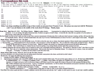
Mohammad's results 2014_02_15: Experimental Result of Addition: Data size: 1 billion, 2 billion, 3 billion, 4 billion. Number of columns: 2 Bit width of the values: 4 bit, 8 bit, 12 bit and 16 bit . Vertical axis is time measured in millisecond. Horizontal axis is number of bit positions.
Y(.15) {y6,y7,y8,y9,ya}(.17) {y7,8,9,a}(.39) {y7,y8,y9,ya}(.39) {yb,yc,yd,ye,yf}(.25) {yb,yc,yd,ye}(1.01) {yb,yc,yd,ye}(1.01) {ya}() {y5}() {y4}() {y1,y2,y3,y4}(.63) {y7,y8,y9}(1.27) {y1,y2,y3}(2.54) {y6,yf}(.08) {y6,yf}(.08) {y7,y8,y9,ya,yb.yc.yd.ye}(.07) {y7,y8,y9,ya,yb.yc.yd.ye}(.07) {y1,y2,y3,y4,y5}(.37) y1,2,3,4,5(.37 {y6}() {yf}() {y6}() {yf}() {y6,y7,y8,y9,ya,yb.yc.yd.ye,yf}(.09) {y1,y2,y3,y4,y5}(.37) 123456789abcdef {yf}() {yb,yc,yd,ye}(1.01) {y6}() {y7,y8,y9,ya}(.39) APPLYING FAUST GAP Clusterer TO SPAETH DensityCount/r2 labeled dendogram for FAUST GAP Cluster on Spaeth with D=Avg-to-Furthest and DensityThreshold=.3 1 3 1 0 2 0 6 2 D=Avg-to-Furthest cut at 7 and 11 1 y1y2 y7 2 y3 y5 y8 3 y4 y6 y9 4 ya 5 6 7 8 yf 9 yb a yc b yd ye c d e f 0 1 2 3 4 5 6 7 8 9 a b c d e f D=Avg-to-Furth DensityThresh=.5 D=Avg-to-Furth DensityThresh=1 D-line Labeled dendogram for FAUST Cluster on Spaeth with D=furthest-to-Avg, DensityThreshold=.3 1 y1y2 y7 2 y3 y5 y8 3 y4 y6 y9 4 ya 5 6 7 8 yf 9 yb a yc b yd ye 0 1 2 3 4 5 6 7 8 9 a b c d e f DCount/r2 labeled dendogram for FAUST Gap Cluster on Spaeth w D=cylces thru diagonals nnxx,nxxn,nnxx,nxxn..., DensThresh=.3 Y(.15) Y(.15)
FAUST ClassifiersFAUST = Fast, Analytic, Unsupervised and Supervised Technology C = class, X = unclassified samples, r = a chosen minimum gap threshold. FAUST One-Class Spherical (OCS) FAUST Multi-Class Spherical (MCS) Classify x as class C iff the count of cCk s.t.(c-x)o(c-x) r2 is max Classify x as class C iff there exists cC such that (c-x)o(c-x) r2 a a a a a a a a aa a a a a aa a c c c c c c c c cc c c c c cc c b b b b b b b b bb b b b b bb b D=e1+e2+e3 D=e1-e3 e3 e2 D=e1+e3 e1 mxCoD12 mnCoD12 mnC1 mxC1 mnA1 mnB1 mxB1 mxA1 mxBoD12 mnBoD12 mxAoD12 mnAoD12 FAUST One-Class Linear (OCL)Construct a hull, H, around C. x is class C iff xH. For a series of vectors, D, let loDmnCoD (or the 1st PCI); hiDmxCoD (or the last PCD). Classify xC iff loD Dox hiD D. E.g., let the D-series be the diagonals e1, e2, ...en, e1+e2, e1-e2, e1+e3, e1-e3, ...,e1-e2-...-en? (add more Ds until diamH-diamC < ε? FAUST Multi-Class Linear (MCL)Construct a hull, Hk, about Ck k as above. Then x isa Ck iff k, xHk. (allows for a "none of the classes" when xHk, k.) The Hks can be constructed in parallel: Convex hull Our hull, H c c c c c c c c cc c c c c cc c D12=e1-e2 line 3D example of HULL1 e1 line 1-class classification Reference : http://homepage.tudelft.nl/n9d04/thesis.pdf#appendix*.7