Regional Coastal Ocean Modeling: Tutorial
Regional Coastal Ocean Modeling: Tutorial. Roms_tools. System requirements. F95 (ifort), Matlab Netcdf library for Fortran and Matlab (MexCDF) 2 Gbites of disk space ROMS_AGRIF sources Matlab toolbox for ROMS: ROMS_tools

Regional Coastal Ocean Modeling: Tutorial
E N D
Presentation Transcript
Regional Coastal Ocean Modeling: Tutorial Roms_tools Patrick Marchesiello IRD 2005
System requirements • F95 (ifort), Matlab • Netcdf library for Fortran and Matlab (MexCDF) • 2 Gbites of disk space • ROMS_AGRIF sources • Matlab toolbox for ROMS: ROMS_tools • Data: bathymetry, hydrography, surface fluxes global climatological datasets are included Patrick Marchesiello IRD 2005
Package Patrick Marchesiello IRD 2005
Pre-processing data • % cd ~/Roms_tools/Run • % matlab • >> start adds the path of different toolboxes • >> make_grid • >> make_forcing • >> make_clim • >> make_tides • >> make_biol • >> nestgui Patrick Marchesiello IRD 2005
% % Title % title='Peru Test Model'; % % Grid file name % grdname='roms_grd.nc'; % % Grid dimensions: % lonmin=-85; lonmax=-75; latmin=-15; latmax=-7; % % Grid resolution [degree] % dl=1/3; % % Minimum depth [m] % hmin=10; % % Topography netcdf file name (ETOPO 2) % topofile='../Topo/etopo2.nc'; % % Slope parameter (r=grad(h)/h) maximum value for topography smoothing % rtarget=0.2; make_grid.m lon, lat, dx, dy, h L=31 M=26 h Patrick Marchesiello IRD 2005
Smoothing methods • r = Δh / h is the slope of the logarithm of h • One method (ROMS): smoothingln(h) until r < rmax Res: 1 km r < 0.25 Res: 5 km r < 0.25 Senegal Bathymetry Profil Patrick Marchesiello IRD 2005
Smoothing method and resolution Bathymetry Smoothing Error off Senegal Convergence at ~ 4 km resolution Standard Deviation [m] Grid Resolution [deg] Patrick Marchesiello IRD 2005
Errors in Bathymetry data compilations Gebco1 compilation Etopo2: Satellite observations Shelf errors (noise) Patrick Marchesiello IRD 2005
Refine the mask • >> editmask • Interactive matlab tool to modify masking according to high resolution coastline data Patrick Marchesiello IRD 2005
Getting the wind forcing • >> make_forcing % % Title - Grid file name - Forcing file name % title='Forcing (COADS)'; grdname='roms_grd.nc'; frcname='roms_frc.nc'; % % % Set times and cycles: monthly climatology for all data % time=[15:30:345]; % time cycle=360; % cycle Default COADS climatological surface forcing of Da Silva et al., 1994 Patrick Marchesiello IRD 2005
Modified Julian dates • MJD is a modification of the Julian Date that is routinely used by astronomers, geodesists, and even some historians. • This dating convention, designed to facilitate chronological calculations, numbers all days in consecutive fashion, beginning so as to precede the historical period. • Julian Day Number 0 is noon 1 January 4713 B.C. • MJD modifies this Julian Date in two ways. • The MJD begins at midnight rather than noon, in keeping with more standard conventions. • Secondly, for simplicity, the first two digits of the Julian Date are removed. This is because, for some three centuries following 17 November 1858, the Julian day lies between 2400000 and 2500000. The MJD drops those first "24" digits. Thus, we have • MJD = JD - 2400000.5 • To convert Julian Dates to Gregorian dates (month/day/year) we can use various converters Patrick Marchesiello IRD 2005
Getting the lateral boundary conditions % % Title % title='Climatology'; % % Switches for selecting what to process (1=ON) % makeclim=1; %1: process boundary data makeoa=1; %1: process oa data makeini=1; %1: process initial data % % Grid file name - Climatology file name % Initial file name - OA file name % grdname ='roms_grd.nc'; frcname ='roms_frc.nc'; clmname ='roms_clm.nc'; ininame ='roms_ini.nc'; oaname ='roms_oa.nc'; % % Vertical grid parameters % theta_s=7.; theta_b=0.; hc=5.; N=20; % number of vertical levels (rho) • >> make_clim OA (objective analysis) files are intermediate files where hydrographic data are interpolated (extrapolated under bathymetry) and stored on a horizontal grid but on z vertical grid. The transformation to S-coordinate is done after. Patrick Marchesiello IRD 2005
obc=[1 0 1 1]; % open boundaries (1=open , [S E N W]) % % Level of reference for geostrophy calculation % zref=-500; % % Day of initialization % tini=15; % % Set times and cycles: monthly climatology for all data % time=[15:30:345]; % time cycle=360; % cycle % % Data climatologies file names: % temp_month_data ='../WOA2001/temp_month.cdf'; temp_ann_data ='../WOA2001/temp_ann.cdf'; insitu2pot=1; % transform in-situ temperature to potential temperature salt_month_data ='../WOA2001/salt_month.cdf'; salt_ann_data ='../WOA2001/salt_ann.cdf'; % Patrick Marchesiello IRD 2005
Getting the tides boundary conditions % % TPXO file name % tidename='../Tides/TPXO6.nc'; % % ROMS file names % gname = 'roms_grd.nc'; fname = 'roms_frc.nc'; % % Number of tides component to process % Ntides=10; % % Set start time of simulation % year = 2000; month = 1; day = 15; hr = 0.; minute = 0.; second = 0.; • >> make_tides This is where tidal information is added This is the starting time of simulation. A procedure correct phases and amplitudes (nodal corrections) for real time runs. It employs parts of a post-processing code from Egbert and Erofeeva (2002) TPXO model. Running Real-time tides requires using modified julian dates as initial time (roms_ini.nc). Patrick Marchesiello IRD 2005
Getting child grids for nesting • >> nestgui Patrick Marchesiello IRD 2005
Preparing the model • % vi param.h • % vi cppdefs.h • Define CPP keys that used by the C-preprocessor when compiling the model • Reduce code to its minimal size: fast compilation • Avoid fortran logical statements: efficient coding parameter (LLm0=29, MMm0=24, N=20) ! Peru Test Case Patrick Marchesiello IRD 2005
PERU : Configuration Name, this is used in param.h. • OPENMP : Activate Open-MP parallelization protocol. • MPI : Activate MPI parallelization protocol. • AGRIF : Activate the nesting capabilities • SOLVE3D : Define if solving 3D primitive equations • UV_COR : Activate Coriolis terms. • UV_ADV : Activate advection terms. • SSH_TIDES : Define for processing sea surface elevation tidal data at the model boundaries. • UV_TIDES : Define for processing ocean current tidal data at the model boundaries. • VAR_RHO_2D : Activate nonuniform density in barotropic mode pressure- gradient terms. • FLAT_WEIGHTS : Use a more dissipative averaging for the baroclinic/barotropic coupling. • CURVGRID : Activate curvilinear coordinate grid option. • SPHERICAL : Activate longitude/latitude grid positioning. • MASKING : Activate land masking in the domain. • AVERAGES : Define if writing out time-averaged data. • SALINITY : Define if using salinity. • NONLIN_EOS : Activate the nonlinear equation of state. • SPLIT_EOS : Activate to split the nonlinear equation of state in a adiabatic part and a compressible part. • ZCLIMATOLOGY : Activate processing of sea surface height climatology. • UCLIMATOLOGY : Activate processing of momentum climatology. • ZNUDGING : Activate open boundary passive/active term + nudging layer for zeta. • M2NUDGING : Activate open boundary passive/active term + nudging layer for ubar and vbar. • SPONGE : Activate areas of enhanced viscosity/diffusion. • … Patrick Marchesiello IRD 2005
Input parameter file title: PERU TEST MODEL time_stepping: NTIMES dt[sec] NDTFAST NINFO 720 1800 45 1 S-coord: THETA_S, THETA_B, Hc (m) 7.0d0 0.0d0 5.0d0 grid: filename roms_grd.ncforcing: filename roms_frc.ncclimatology: filename roms_clm.ncinitial: NRREC filename 1 roms_ini.ncrestart: NRST, NRPFRST / filename 720 -1 roms_rst.nchistory: LDEFHIS, NWRT, NRPFHIS / filename T 144 0 roms_his.ncaverages: NTSAVG, NAVG, NRPFAVG / filename 1 144 0 roms_avg.ncprimary_history_fields: zeta UBAR VBAR U V wrtT(1:NT) T F F T T 10*Tauxiliary_history_fields: rho Omega W Akv Akt Aks HBL Bostr F F F F T F T Fprimary_averages: zeta UBAR VBAR U V wrtT(1:NT)T T T T T 10*Tauxiliary_averages: rho Omega W Akv Akt Aks HBL F T F F T F T • % vi roms.in rho0: 1025.d0lateral_visc: VISC2, VISC4 [m^2/sec for all]0. 0.tracer_diff2: TNU2(1:NT) [m^2/sec for all] 10*0.d0 bottom_drag: RDRG [m/s], RDRG2, Zob [m], Cdb_min, Cdb_max 3.0d-04 0.d-3 0.d-3 1.d-4 1.d-1 gamma2: 1.d0sponge: X_SPONGE [m], V_SPONGE [m^2/sec] 150.e3 500.nudg_cof: TauT_in, TauT_out, TauM_in, TauM_out [days for all] 1. 360. 3. 360. Patrick Marchesiello IRD 2005
Compiling the model • % jobcomp • Automatic selection of compilation options according to the plateform • Set library path • Use Makefile: • C-preprocessing: file.F file.f • Compiling: file.f file.o • Links with libraries executable roms Patrick Marchesiello IRD 2005
Preparing AGRIF • % vi AGRIF_FixedGrids.in 2 20 45 34 59 3 3 3 30 55 70 89 3 3 2 0 1 10 30 20 40 5 3 5 0 1 20 33 34 44 3 3 3 PERU test case Patrick Marchesiello IRD 2005
Running the model MAIN: started time-steping. STEP time[DAYS] KIN_EN POT_EN TOTAL_EN NET_VOLUME trd 0 15.00000 0.000000000E+00 2.5311945E+01 2.5311945E+01 2.2335422E+15 0 1 15.02083 3.332338732E-06 2.5312150E+01 2.5312154E+01 2.2335431E+15 0 2 15.04167 1.062963402E-05 2.5312316E+01 2.5312327E+01 2.2335455E+15 0 3 15.06250 2.075678260E-05 2.5312446E+01 2.5312466E+01 2.2335461E+15 0 4 15.08333 3.186463589E-05 2.5312543E+01 2.5312575E+01 2.2335469E+15 0 5 15.10417 4.285427484E-05 2.5312627E+01 2.5312670E+01 2.2335480E+15 0 6 15.12500 5.333102059E-05 2.5312691E+01 2.5312744E+01 2.2335479E+15 0 7 15.14583 6.354045596E-05 2.5312719E+01 2.5312782E+01 2.2335465E+15 0 8 15.16667 7.411816854E-05 2.5312701E+01 2.5312775E+01 2.2335457E+15 0 9 15.18750 8.562138804E-05 2.5312650E+01 2.5312735E+01 2.2335467E+15 0 10 15.20833 9.828165268E-05 2.5312569E+01 2.5312667E+01 2.2335473E+15 0 11 15.22917 1.117146701E-04 2.5312465E+01 2.5312577E+01 2.2335475E+15 0 12 15.25000 1.255576462E-04 2.5312345E+01 2.5312471E+01 2.2335475E+15 0 13 15.27083 1.393087941E-04 2.5312135E+01 2.5312275E+01 2.2335470E+15 0 14 15.29167 1.525558114E-04 2.5311800E+01 2.5311952E+01 2.2335463E+15 0 15 15.31250 1.653985076E-04 2.5311350E+01 2.5311515E+01 2.2335465E+15 0 16 15.33333 1.779958127E-04 2.5310792E+01 2.5310970E+01 2.2335468E+15 0 17 15.35417 1.905668926E-04 2.5310134E+01 2.5310325E+01 2.2335470E+15 0 18 15.37500 2.034591092E-04 2.5309385E+01 2.5309588E+01 2.2335470E+15 0 19 15.39583 2.165195050E-04 2.5308554E+01 2.5308771E+01 2.2335469E+15 0 20 15.41667 2.294900067E-04 2.5307653E+01 2.5307882E+01 2.2335465E+15 0 21 15.43750 2.422211112E-04 2.5306695E+01 2.5306937E+01 2.2335463E+15 0 22 15.45833 2.545401621E-04 2.5305693E+01 2.5305948E+01 2.2335463E+15 0 23 15.47917 2.664383353E-04 2.5304665E+01 2.5304932E+01 2.2335464E+15 0 24 15.50000 2.780681955E-04 2.5303629E+01 2.5303907E+01 2.2335465E+15 0 25 15.52083 2.896947197E-04 2.5302600E+01 2.5302890E+01 2.2335465E+15 0 26 15.54167 3.013595537E-04 2.5301595E+01 2.5301897E+01 2.2335462E+15 0 % roms roms.in Patrick Marchesiello IRD 2005
Visualizing the results >> roms_gui Patrick Marchesiello IRD 2005
Analysing the results • Make statistics (mean, variance, …) • Use tracers, compute residence times and Lagrangian transport • Make budgets (energy, heat, vorticity, momentum, …) • Comparison with available data • … Patrick Marchesiello IRD 2005