Decomposing a time series
Decomposing a time series. (Session 03). Learning Objectives. By the end of this session, you will be able to explain the form of two typical models for a time series make a decision concerning whether to use an additive or multiplicative model estimate the seasonal effect in a series

Decomposing a time series
E N D
Presentation Transcript
Decomposing a time series (Session 03)
Learning Objectives By the end of this session, you will be able to • explain the form of two typical models for a time series • make a decision concerning whether to use an additive or multiplicative model • estimate the seasonal effect in a series • explain how to de-seasonalise the series and use of such a series
Recall classical decomposition • Trend (Tt) - Long term movement in the mean • Seasonal variation (St) – Short-term fluctuations, usually within a year (we will assume this in what follows) • Cycles (Ct) – Long-term cyclical patterns e.g. sun-spots, business cycles • Residuals (Et) - random and all other unexplained components of variation
A model for the series We will not be considering the cyclical component in this module. In this session we look at seasonal effects. For this, need to decide whether the series is better represented by an Additive model, i.e. Datat = Tt + St + Rt OR by a Multiplicative model, i.e. Datat = Tt x St x Rt Here Tt , St and Rt are called the trend, seasonal and residual effects respectively.
An example Monthly tourist arrivals in Sri Lanka from 1968–1971. Notice the slight increase in variation over time. This requires using a multiplicative model.
Additive or Multiplicative? • In an additive model, the seasonal effect is the same (roughly constant) in the same period over different years • Sometimes the seasonal effect is a proportion of the underlying trend value, e.g. in previous slide, they increase as the trend increases • It is then appropriate to use a multiplicative model
Estimating the seasonal effect • Recall that the seasonal effects occur when the series repeats systematically in short periods (often within a year) of time • Seasonal effects need to be removed before we can compare similar time periods in different seasons • A brief outline is presented in the next slide - with a numerical example discussed thereafter
Estimating the seasonal effect • First de-trend the series by finding either Di = Yi – Ti or Di = Yi/Ti • The seasonal means are then obtained as the averages of the detrended values Di • They are then scaled so that the seasonal mean (a) averages to zero for an additive model, or (b) averages to 1 for a multiplicative model. The example in the handout entitled “Estimating trends and seasonal effects” will now be discussed to show the steps involved. Used here will be data on unemployed school leavers (same as in Session 02)
De-seasonalising the series • Like de-trending, may also de-seasonalise the series by removing the seasonal effect • For an additive model, the de-seasonalised series is obtained as Di = Yi – Si • For a multiplicative model, the de-seasonalised series is obtained as Di = Yi/Si • A de-seasonalised series shows the pattern of change over time with all seasonal effects removed. This allows direct comparisons between time points in this series, unaffected by seasonal changes.
Practical work • Use again the data on unemployed school leavers, to estimate the seasonal effect using an additive model. (See Practical 3) • Go through parts of Section 2.3 of CAST for SADC : Higher Level with a view to improving your understanding of ideas covered in this session.

