SOURCE TIME SERIES
SOURCE TIME SERIES. VOCAL TRACT TRANSFER FUNCTION. VOICE TIME SERIES. VOICE SPECTRUM. CASE 0: NORMAL SOURCE AND NORMAL VOCAL TRACT. CASE 1: “BREATHY” SOURCE AND NORMAL VOCAL TRACT. SOURCE TIME SERIES. VOCAL TRACT TRANSFER FUNCTION. VOICE TIME SERIES. VOICE SPECTRUM.

SOURCE TIME SERIES
E N D
Presentation Transcript
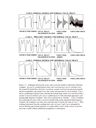
SOURCE TIME SERIES VOCAL TRACT TRANSFER FUNCTION VOICE TIME SERIES VOICE SPECTRUM CASE 0: NORMAL SOURCE AND NORMAL VOCAL TRACT CASE 1: “BREATHY” SOURCE AND NORMAL VOCAL TRACT SOURCE TIME SERIES VOCAL TRACT TRANSFER FUNCTION VOICE TIME SERIES VOICE SPECTRUM CASE 2: NORMAL SOURCE AND ABNORMAL VOCAL TRACT SOURCE TIME SERIES VOCAL TRACT TRANSFER FUNCTION VOICE TIME SERIES VOICE SPECTRUM Figure 3.1. Ambiguity between the source and vocal tract models is illustrated with three examples. In case 0, a normal glottal source and vocal tract give rise to a normal voice; the normal LF glottal flow derivative waveform, normal vocal tract log spectrum transfer function magnitude, and normal voice time series and spectrum for /a/ are plotted. Case 1 shows a pathological glottal source missing the normal sharp return; it is convolved with a normal vocal tract model to give rise to a pathological /a/ with sinusoidal appearance and missing high frequency formants. This voice is perceived as “breathy.” Case 2 combines the normal glottal source with a vocal tract model with greatly attenuated high frequency formants; the resulting voice time series and spectrum is exactly the same as case 1. Thus, working backwards from the resulting time series of cases 1 and 2 (as is attempted in inverse filtering and formant analysis), it is impossible to arrive at the correct vocal tract and source model without additional assumptions or information.
PC #1: STIMULUS GEN. STIMULUS SIGNAL D/A ACOUSTIC CONDUIT /a/ AMPLIFIER XDUCER PC #2: DAQ CH 1 SIGNAL CONDITIONER A/D MEM. MICROPHONE VOCAL TRACT CH 2 SIGNAL CONDITIONER A/D TUBE OF LENGTH L WITH CLOSED END. FORMANTS AT F = C/4L, 3C/4L, 5C/4L,... Figure 3.2. System setup for external stimulation of the vocal tract. Two PCs are used: PC #1 generates a stimulus signal to excite the vocal tract. An audio amplifier and transducer transform the stimulus to sound, which is then conducted via an acoustic conduit to either a quarter wave tube model or the subject’s vocal tract. PC #2 is used to record the stimulus and response signals. A sample of the stimulus is acquired on channel 1 of an analog to digital converter and is stored to memory. The response is recorded with a small microphone, conditioned and acquired on channel 2 of the analog to digital converter. The tube model is used for proof of principle and system validation.
A/D CH 1 x(t) EXTERNAL STIMULUS AMP & XDCR DYNAMICS H1(s) ROOM/FACE ACOUSTICS H2(s) S0 A/D CH 2 S1 + g(t) MIC & SIG COND. H3(s) GLOTTAL SOURCE VOCAL TRACT V(s) r(t) S2 + Figure 3.3. Model of external source formant analysis system. In addition to the normal glottal source g(t) and vocal tract V(s) pathway, an external source x(t) is added to stimulate the vocal tract. Stimulus electronics, transducer, and environmental acoustics are modeled in H1 and H2; microphone and signal conditioning are modeled in H3. Switches S0 and S2 represent presence/absence of x(t) and g(t); S1 represents presence/absence of the vocal tract (mouth open or shut).
SPECTRUM WITH RAG, W/O RAG, & MAG OF T.F. 140 |HA(f)| 120 |HB(f)| 100 80 60 TUBE FORMANTS MAGNITUDE (dB) 40 20 0 -20 -40 |V(f)| -60 0 0.2 0.4 0.6 0.8 1 1.2 1.4 1.6 1.8 2 FREQUENCY (Hz) 4 x 10 Figure 3.4. Validation of external source testing setup using a simple quarter wave tube closed at one end. HA is the spectrum recorded by the microphone near the open end of the tube when a 0 – 10KHz stimulus sinewave sweep is executed. HB is the “background” spectrum recorded when the tube is stuffed with a rag, effectively eliminating the tube formants. V is HA – HB, revealing the expected quarter wave tube formants. All spectra become noise above 10KHz at the end of the sweep.
140 MOUTH SHUT FREQ. RESP. 120 100 MOUTH OPEN FREQ. RESP. 80 60 MAGNITUDE (dB) 40 VOCAL TRACT FREQ. RESP. 20 0 -20 0 500 1000 1500 2000 2500 3000 3500 4000 4500 5000 FREQUENCY (Hz) Figure 3.5. Vocal tract transfer function for /a/ with a normal male voice. Analogous to Fig 3.4, the chirp response spectra of mouth open/shut (top curves) are subtracted to yield the vocal tract frequency response (bottom). The expected formants for /a/ are present, plus additional peaks. Ripples at 94 Hz spacing in the top curves due to acoustic conduit resonances are effectively cancelled by the subtraction process.
COMPARE TF USING MOUTH OPEN SWEEP1 VS SWEEP2 30 25 20 F1 F2 F3 F4 15 10 5 MAGNITUDE (dB) 0 -5 -10 -15 -20 0 500 1000 1500 2000 2500 3000 3500 4000 4500 5000 FREQUENCY (Hz) Figure 3.6. Drift in formant peaks during testing. In order to estimate effects of articulator movements, the vocal tract calculation is repeated using different chirps from the same time series. In this case, the peaks remained fairly constant with about 100 Hz change at 3200 Hz ( 3% ).
F1 F2 20 EXT SRC T.F.’S 10 0 -10 F3 F4 -20 LP -30 MAGNITUDE (dB) -40 -50 -60 -70 FFT -80 0 500 1000 1500 2000 2500 3000 3500 4000 4500 5000 FREQUENCY (Hz) Figure 3.7. Comparison of traditional FFT/LP analysis with the ES analysis of Fig. 3.5. Formant peak shifts between FFT/LP and ES resonances are probably due to involuntary articulator movement from the vocalizing to non-vocalizing transition. Many resonances are shown in the ES data that are not revealed by FFT/LP.
VOCALIZING /a/ MIC SIGNAL (TOP), EXT. SRC (BOT) MIC SIGNAL 2 MOUTH OPEN MOUTH SHUT 1.5 1 0.5 PULSE+CHIRP EXTERNAL SOURCE 0 SIGNALS -0.5 -1 -1.5 -2 0 0.5 1 1.5 2 2.5 3 3.5 4 4.5 TIME (SEC) Figure 3.8. Time history of vocal tract audio output (top) and the ES (external source) stimulus (bottom). Periodic pulse + sine chirps are interspersed with periods of silence, during which vocalization (alone) can be recorded (0.3 s to 0.8 s). The resonances of the vocal tract are clearly visible in the mouth open responses at 1.7 s and 2.6 s. Note that the first chirp occurs during vocalizing; this was done to allow collection of data for future analysis using correlation techniques to separate the responses to chirp and glottis.
EXT SRC T.F.’S 30 F1 F2 20 10 0 -10 F3 F4 -20 MAGNITUDE (dB) LP -30 -40 -50 -60 -70 FFT -80 0 500 1000 1500 2000 2500 3000 3500 4000 4500 5000 FREQUENCY (Hz) Figure 3.9. FFT/LP/ES analysis of another instance of normal male /a/. Compare with Fig 3.9b which is a breathy /a/ from the same time series.
30 EXT SRC T.F.’S 20 F1 F2 10 0 -10 F3 F4 -20 MAGNITUDE (dB) LP -30 -40 -50 -60 FFT -70 -80 0 500 1000 1500 2000 2500 3000 3500 4000 4500 5000 FREQUENCY (Hz) Figure 3.9b. FFT/LP/ES analysis of a breathy /a/ from the same time series as Fig. 3.9.
BREATHY /a/ MODAL /a/ 2 MOUTH OPEN MIC SIGNAL MOUTH SHUT 1.5 1 0.5 PULSE+ CHIRP EXTERNAL SOURCE NORMALIZED SIGNAL 0 -0.5 -1 -1.5 -2 0.5 1 1.5 2 2.5 SAMPLE # FSR=44100 5 x 10 Figure 3.10. Time history of vocal tract output and ES (analogous to Fig. 3.8) with an added breathy segment at the beginning. The voice is the author’s.
30 F1 F2 20 EXT SRC T.F. 10 0 -10 F3 F4 -20 MAGNITUDE (dB) -30 LP -40 -50 -60 FFT -70 -80 0 500 1000 1500 2000 2500 3000 3500 4000 4500 5000 FREQUENCY (Hz) Figure 3.11. FFT/LP/ES analysis of a normal female /a/. Compare to Fig 3.11b which contains a breathy /a/ from the same time series.
30 F1 F2 20 EXT SRC T.F. 10 0 -10 F4 F4 -20 MAGNITUDE (dB) LP -30 -40 -50 -60 FFT -70 -80 0 500 1000 1500 2000 2500 3000 3500 4000 4500 5000 FREQUENCY (Hz) Figure 3.11b. FFT/LP/ES analysis of a female breathy /a/. Compare to Fig 3.11 which contains a normal /a/ from the same time series.