Download
1 / 15
150 likes | 349 Vues
Summarizing the Relationship Between Two Variables with Tables and a bit of a review. Chapters 6 and 7 Jan 31 and Feb 1, 2012. Looking at Tables . Tables are useful for examining the relationship between: variables measured at the nominal or ordinal level,

E N D
Summarizing the Relationship Between Two Variables with Tables and a bit of a review Chapters 6 and 7 Jan 31 and Feb 1, 2012
Looking at Tables • Tables are useful for examining the relationship between: • variables measured at the nominal or ordinal level, • or variables measured at the interval or ratio level with a small number of discrete values.
Some Terminology and Conventions • Two-way tables, Crosstabulations (Crosstabs) • Column (explanatory or independent) • Row (response or dependent) • Although the book does not always do this, there is a soft convention of stating a table title as “Dependent by Independent”. E.g. Table 2: Election Needed Now by Province.
Cells: As in a spread sheet a table is divided into cells aligned along rows and columns. • Marginal Distributions: These are the numbers that summarize the rows and the columns at the side and bottom of a table • Conditional Distributions: The book gives a very complicated explanation for what this is. In reality it is just the percentage of the cases in a cell or cells. This can be the percentage of cases along the horizontal row or the vertical column.
Here is an example of a Two Way table made with the “crosstab” procedure in SPSS (see my tip sheet for doing them in Excel). Question. Is there a difference between the number of bathrooms that homes in urban and rural Ontario have? • Look at row 1. Reading Across: we see 94% of the homes with 1 bathroom are Urban 6% are Rural • Look at Column 1. Reading Down: we see 52.2% of urban homes have 1 bath-room, 36.8% have 2 bathrooms 11.0% have three or more bathrooms.
The percentages give us a way to ‘eyeball’ the data and estimate if there is a difference, but to ask if these difference are meaningful, we must go further and calculate some statistics.
The Chi Sq. Test is a common one to use in a table with nominal variables such as this. • It measures the difference between the number of cases we expect to see in each cell and the number of cases we actually observe in each cell of our table. • The Chi Sq. value itself has little meaning for us. What matters is whether or not the value is significant. In this case it is > .05. • Therefore we reject the hypothesis that the results we see are meaningfully different from what we could expect through simple probability • Therefore we also reject that there is any meaningful difference between the number of bathrooms in urban and rural homes.
Simpson’s ParadoxThat lurking variable thing again • Example 6.4 in your book gives you a look at a problem called Simpson’s Paradox. • An association or comparison that holds for all or several groups can reverse direction when the data are combined to form a single group (Moore pg. 169). • As Moore further notes, this is usually the sign of a “lurking” variable.
In order to check for lurking variables we can subdivide tables by a further categorical variable (such as was done in the book where the data was divided into serious and less serious accidents).
The book has two very nice “four step” graphics in Chapter 7
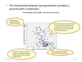
I would probably adjust this a bit. • In the final leg I would say: • If the Y (response or dependent) variable is quantitative (measured at the interval or ratio level) a regression line is a good summary. • However, if the Y (response or dependent) variable is ordinal or nominal, then a two way table is needed.
And again the general four step approaches to any statistical problem • State: What is the practical question, in the context of the real world setting • Plan: What specific statistical operations does this problem call for • Solve: Make the graphs and carry out the calculations needed for this problem • Conclude: Give your practical conclusion in the setting of the real-world problem
Also keep in mind… • I would also remind you that we looked at a couple of things the book did not cover, such as “spearman’s rho” as an alternative measure of correlation when working with a table in which both variables are ordinal and Chi Sq.