Download
1 / 38
380 likes | 571 Vues
Recap on biological oceanography. Oceans Biosphere Rock Weathering. CO 2. changes in the last 50 yr. Carbon Cycle. from dissolution of Calcium Carbonate. The Carbonate System. sources of inorganic carbon. from dissolved CO 2 gas. Total dissolved inorganic carbon.

E N D
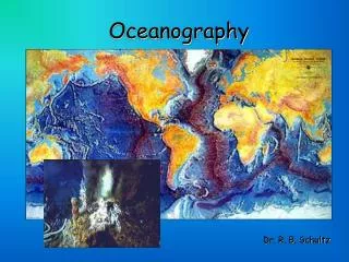
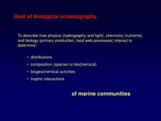
Recap on biological oceanography
Oceans Biosphere Rock Weathering CO2 changes in the last 50 yr
from dissolution of Calcium Carbonate The Carbonate System sources of inorganic carbon from dissolved CO2 gas Total dissolved inorganic carbon
Carbon Dioxide and Carbonate system Carbonic Acid Bicarbonate Ion Carbonate
O2 CO2 pH (m) acid basic
compensation depth low oxygen environment Respiration: Animal, plants and microbial decomposition Dissolved Gases in the Ocean Oxygen profile
- + Distribution of Carbon species in water
Higher CO2 levels will generally be detrimental to calcifying organisms and that food web structures and biodiversity will likely change, Corals Coccolithophores Forams calcite calcite aragonite but it is not clear how this might impact overall productivity and top level predators (e.g. fish).
Biogeochemical Controls and Feedbacks on the Ocean Primary Production 3) Subpolar Gyres 2) Upwelling Regions 1) Subtropical Gyres 4) HNLC regions What can explain the chlorophyll distribution?
What are the controls on Export Production? • Ocean nutrient inventory Nitrogen appears to be the control duringmodern time. Where nitrogen can be brought at the surface there is higher productivity: Upwelling regions and subpolar gyres Exception: HNLC regions, particularly in the Southern ocean The Iron Problem
Southern Ocean HNLC Map of annual average nitrate concentrations in the surface waters of the oceans. Data from Levitus, World Ocean Atlas, 1994.
Advanced Very High Resolution Radiometer (AVHRR) images of particle transport in the atmosphere between June and August.
Biophysical interactions • Wind-driven gyre circulation for surface distributions; • MOC for concentrations at depth
North-south sections of (a) temperature, (b) salinity, and (c) oxygen along the 30oW transect in the Atlantic ocean. Note the salinity tongues indicating the interleaving of water masses from sources in the Antarctic and the North Atlantic.
Summaring • The large scale wind-driven circulation explains the (large scale) distribution of chlorophyll. • We need to consider the biology to explain the distribution of nitrate (remember the high latitudes and the iron problem!) • The thermohaline circulation explains the vertical distributions of oxygen and NO3 and the differences between the basins at depth
The Nitrogen Cycle • The Demand Side. • Denitrification. • Alternative pathways to N2. • The Supply Side • Nitrogen Fixation: the usual suspects. • “New” diazotrophs and how they work.
Who Cares? • Broad reaches of the ocean are N-limited. • Recycling of N within the water column supports biological production, but… • Injection of new N into the upper water column is required to support export production. • The N and C cycles are tightly coupled through biological production of organic matter (C:N ≈ 7). • The N cycle therefore plays a key role in regulating the C cycle!
Oceanic N Cycle Schematic Fixation N2 Nitrification Mineralization NH4 NO3 Uptake Phytoplankton Grazing Mix Layer depth Chlorophyll Zooplankton Mortality Large detritus Water column Susp. particles Nitrification N2 NH4 NO3 Denitrification Aerobic mineralization Organic matter Sediment
Major Biological Transformations of Nitrogen (Inspired by Codispoti 2001and Liu 1979)
The major oceanic inputs and outputs of combined N are largely separated in space. • Denitrification is restricted to sediments and anoxic water masses. • N2-fixation is common in oligotrophic surface waters (e.g., the central gyres of the major ocean basins).
N* Distribution Shows Interplay Between N2-Fixation and Denitrification N* = 0.87( [NO3-] - 16[PO43-] + 2.9) (Gruber & Sarmiento 1997)
What else? • Time-dependence: waves, eddies, convection, ocean-atmosphere interactions and various modes of variability from intraseasonal to inderdecadal (ENSO, NAO, PDO, NPGO ….)
La Nina conditions El Nino conditions
in the North Pacific Pacific Decadal Oscillation
Mean Sea Level Pressure Anomaly PDO Negative Phase Anomaly PDO Positive Phase
+ - +
The NPGO (North Pacific Gyre Oscillations) Di Lorenzo et al. GRL 2008 North Pacific dominant mode of oceanic variability: the PDO and NPGO (left), are driven by the first two dominant modes of atmospheric variability evident in sea level pressure, the Aleutian Low variability and the NPO.
Variability of subsurface nitrate (NO3). (A) Mean subsurface (150m) NO3 from ROMS model over 1975-2004. (B) First mode of variability for model subsurface (150m) NO3 anomaly inferred from EOF1. (C) Timeseries of NPGO index (black) compared to PC1 of NO3 (R=0.65, 99%), observed mix layer NO3 at Line-P [Peña and Varela, 2007], and observed NO3 from CalCOFI program (R=0.51, 95%).
The North Atlantic Oscillation Index The NAO index shows large variations from year to year. This interannual signal was especially strong during the end of the 19th century. Sometimes the NAO index stays in one phase for several years in a row. This decadal variability was quite strong in the second half of the 20th century.
SST Anomalies [C] Positive NAO Wet Stronger Currents more storms Dry Dry Wet fewer storms Weaker Currents Negative NAO
Impacts of the NAO Martin Visbeck