Download
1 / 164
1.64k likes | 1.95k Vues
Explore the fascinating world of binocular disparity and stereopsis, revealing the neural mechanisms behind depth perception and processing of visual stimuli. Learn about disparity-selective neurons and psychophysical limits. Dive into complex cell circuitry and models for depth perception.

E N D
Binocular disparity and Stereopsis Bruce Cumming Laboratory of Sensorimotor Research, National Eye Institute, National Institutes of Health
Put red lens over left eye, blue lens over right eye Stereo anaglyph by Prof. Michael Greenhalgh, Australian National University (with permission).
stereopsis L R
correspondence problem left eye’s image right eye’s image
random-dot patterns • a completely unnatural stimulus • image changes every few ms • no recognisable objects e.g. faces • each dot has dozens of identical potential matches • and yet a clear perception of depth!
Neurons and depth perception • A simple model to generate disparity signals. • How neurons reflect this. • Some psychophysical limits this explains. • Further processing.
head image from Royal Holloway University of London Vision Research Group (with permission)
Right retina Receptive Field Left retina Fovea
* * Disparity-selective neuron Right RF R Left RF L
basic building-block • inner product of image with receptive field Pos(v)
…. ….S= response + 1 + 1 -0.1
=l =r Left RF + S + Right RF
Output (spike rate) l1 r1 r2 l2 l2 r1 Input (membrane V)
BS 2 BS 3 BS 4 Circuitry for complex cell left right binocular simple cells RF1 BS 1 complex cell RF2 Cx If RF2 = -RF 1 in both eyes, then half squaring then summing is equivalent to simply squaring.
square the result sum over many such subunits add together energy model convolution of left eye’s image with jth left receptive field convolution of right eye’s image with jth right receptive field
L R L R Right Stimulus Position Complex cell Left Stimulus Position Model Ohzawa et al, 1990
Disparity-selective neuron Right RF R Left RF L
L R L R L R L R Right Stimulus Position Complex cell Left Stimulus Position Model Ohzawa et al 1990
* * Disparity-selective neuron Right RF R Left RF L
1 0.5 0 -0.5 -1 Left RF Right RF -d d 0 Correlation -50 0 50 Disparity (pixels)
1 0.5 0 -0.5 -1 Patern 1 Patern 2 Patern 3 Patern 4 Correlation Patern 5 Mean -50 0 50 Disparity (pixels)
d -d 0 Disparity
1 0.5 0 -0.5 -1 Right RF Left RF Correlation 0 Disparity
DeAngelis, Ohzawa and Freeman, (1991) Cat simple cell RF maps
For single subunits (simple) • Odd symmetric disparity tuning implies phase disparity • Even symmetry around non-zero disparity implies position disparity True for complex cells if: • All subunits have same phase disparity • All subunits have same position disparity.
Monkey complex cells duf043 duf065 60 40 Firing rate (spikes/s) 20 0 -1.2 -1.0 -0.8 -0.6 -0.4 -0.2 0.0 0.2 0.4 0.6 0.8 0.8 -1.4 -0.9 -0.4 0.1 0.6 1.1 1.4 Disparity (degrees)
So far: • Energy model measures cross-correlation after filtering. • V1 contains a bank of filters measuring these correlations after displacements of both phase and position.
* * Disparity-selective neuron Right RF R Left RF L
the neuronal response cf: 0.06 cpd 80 60 response [spikes/sec] 40 20 0 0 0.5 1 1.5 2 time [sec]
the neuronal response cf: 0.06 cpd 80 60 40 20 0 0 0.5 1 1.5 2 response [spikes/sec] cf: 0.5 cpd 80 60 40 20 0 0 0.5 1 1.5 2 time [sec]
f1 relative modulation corrugation-frequency [cpd] relative modulation cf: 0.06 cpd 80 60 40 f0 20 0 0 0.5 1 1.5 2 response [spikes/sec] cf: 0.5 cpd 80 60 40 20 0 0 0.5 1 1.5 2 time [sec]
SDsf [cpd] SDsf [cpd] SDsf [cpd] SDsf [cpd] SDsf [cpd] SDsf [cpd] SDsf [cpd] SDsf [cpd] SDsf [cpd] SDsf [cpd] RM (f1/f0) RM (f1/f0) RM (f1/f0) RM (f1/f0) RM (f1/f0) RM (f1/f0) RM (f1/f0) RM (f1/f0) RM (f1/f0) RM (f1/f0) sf [cpd] sf [cpd] sf [cpd] sf [cpd] sf [cpd] sf [cpd] sf [cpd] sf [cpd] sf [cpd] sf [cpd] 1/(2πSDrf) [degree-1] 1/(2πSDrf) [degree-1] 1/(2πSDrf) [degree-1] 1/(2πSDrf) [degree-1] 1/(2πSDrf) [degree-1] 1/(2πSDrf) [degree-1] 1/(2πSDrf) [degree-1] 1/(2πSDrf) [degree-1] 1/(2πSDrf) [degree-1] 1/(2πSDrf) [degree-1] response [spikes/sec] response [spikes/sec] response [spikes/sec] response [spikes/sec] response [spikes/sec] response [spikes/sec] response [spikes/sec] response [spikes/sec] response [spikes/sec] response [spikes/sec] vertical position [°] vertical position [°] vertical position [°] vertical position [°] vertical position [°] vertical position [°] vertical position [°] vertical position [°] vertical position [°] vertical position [°] output exponent: 1 2 4 2 1.5 1 corrugation cutoff [cpd] 0.5 0 n=19 r=0.45 0 0.5 1 1.5 2 1/(2*π*SD of RF height) [degree-1]
Predicted from mean V1 response (mean ecentricity 3.7º)
Temporal impulse response (LGN) 10ms Reppas, Usrey and Ried (2000)
drifting luminance grating 80 disparity modulation 1.5 40 40 response [spikes/sec] tf cutoff for drifting luminance grating [Hz] 1 20 relative modulation [f1/f0] 0 n=27 0.5 0 0 20 40 0 tf cutoff for disparity modulation [Hz] 1 10 100 temporal frequency [Hz] temporal frequency [Hz] Temporal frequency tuning for contrast and disparity
Summary • We don’t solve the correspondence problem dot-by-dot. • Is this enough?
1 0.5 0 -0.5 -1 Correlation -50 0 50 RF Disparity (pixels)
1 0.5 0 -0.5 -1 Correlation -50 0 50 RF Disparity (pixels)
P’ P direction of gaze nodal point fovea
Y Z X
Y Z X
Y Z X
probability density function for disparities encountered during natural viewing -15 -10 -5 vertical disparity (degrees) 0 5 10 15 -10 0 10 20 30 horizontal disparity (degrees)
probability density function for disparities encountered during natural viewing -1 -0.5 vertical disparity (degrees) 0 0.5 1 -1 -0.5 0 0.5 1 horizontal disparity (degrees)
-6 -4 -2 0 vertical disparity 2 4 6 -15 -10 -5 0 5 10 15 20 25 30 horizontal disparity