Download
1 / 54
540 likes | 557 Vues
Dive into essential FMRI data analysis techniques and the General Linear Model with Dr. Scott Huettel from Duke University in this week 9 session. Learn about statistical parametric maps, hypothesis-driven analyses, correlation approaches, Fourier analysis, GLM fundamentals, and more. Understand how to interpret your results and generate meaningful insights for your research. Enhance your knowledge with key concepts, experimental designs, regressors, and the optimal use of basis functions in FMRI data analysis discussions. Join this informative course to sharpen your skills and elevate your understanding of data analysis in FMRI studies.

E N D
FMRI Data Analysis:I. Basic Analyses and the General Linear Model FMRI Graduate Course (NBIO 381, PSY 362) Dr. Scott Huettel, Course Director FMRI – Week 9 – Analysis I Scott Huettel, Duke University
When do we not need statistical analysis? Inter-ocular Trauma Test (Lockhead, personal communication) FMRI – Week 9 – Analysis I Scott Huettel, Duke University
Why use statistical analyses? • Replaces simple subtractive methods • Signal highly corrupted by noise • Typical SNRs: 0.2 – 0.5 • Sources of noise • Thermal variation (unstructured) • Physiological, task variability (structured) • Assesses quality of data • How reliable is an effect? • Allows distinction of weak, true effects from strong, noisy effects FMRI – Week 9 – Analysis I Scott Huettel, Duke University
What do our analyses generate? • Statistical Parametric Maps • Brain maps of statistical quality of measurement • Examples: correlation, regression approaches • Displays likelihood that the effect observed is due to chance factors • Typically expressed in probability (e.g., p < 0.001), or via t or z statistics FMRI – Week 9 – Analysis I Scott Huettel, Duke University
What are our statistics for? FMRI – Week 9 – Analysis I Scott Huettel, Duke University
FMRI – Week 9 – Analysis I Scott Huettel, Duke University
Key Concepts • Within-subjects analyses • Simple non-GLM approaches (older) • General Linear Model (GLM) • Across-subjects analyses • Fixed vs. Random effects • Correction for Multiple Comparisons • Displaying Data FMRI – Week 9 – Analysis I Scott Huettel, Duke University
Simple Hypothesis-Driven Analyses • t-test across conditions • Time point analysis (i.e., t-test) • Correlation • Fourier analysis FMRI – Week 9 – Analysis I Scott Huettel, Duke University
Correlation Approaches (old-school) • How well does our data match an expected hemodynamic response? • Special case of General Linear Model • Limited by choice of HDR • Assumes particular correlation template • Does not model task-unrelated variability • Does not model interactions between events FMRI – Week 9 – Analysis I Scott Huettel, Duke University
Fourier Analysis • Fourier transform: converts information in time domain to frequency domain • Used to change a raw time course to a power spectrum • Hypothesis: any repetitive/blocked task should have power at the task frequency • BIAC function: FFTMR • Calculates frequency and phase plots for time series data. • Equivalent to correlation in frequency domain • Subset of general linear model • Same as if used sine and cosine as regressors FMRI – Week 9 – Analysis I Scott Huettel, Duke University
Power 12s on, 12s off Frequency (Hz) FMRI – Week 9 – Analysis I Scott Huettel, Duke University
FMRI – Week 9 – Analysis I Scott Huettel, Duke University
The General Linear Model (GLM) FMRI – Week 9 – Analysis I Scott Huettel, Duke University
Basic Concepts of the GLM • GLM treats the data as a linear combination of model functions plus noise • Model functions have known shapes • Amplitude of functions are unknown • Assumes linearity of HDR; nonlinearities can be modeled explicitly • GLM analysis determines set of amplitude values that best account for data • Usual cost function: least-squares deviance of residual after modeling (noise) FMRI – Week 9 – Analysis I Scott Huettel, Duke University
Signal, noise, and the General Linear Model Amplitude (solve for) Measured Data Noise Design Model Cf. Boynton et al., 1996 FMRI – Week 9 – Analysis I Scott Huettel, Duke University
Form of the GLM Model Functions Model Functions Model * Amplitudes = + Data Noise N Time Points N Time Points FMRI – Week 9 – Analysis I Scott Huettel, Duke University
Design Matrices Model Parameters Images FMRI – Week 9 – Analysis I Scott Huettel, Duke University
Regressors (How much of the variance in the data does each explain?) Contrasts (Does one regressor explain more variance than another?) FMRI – Week 9 – Analysis I Scott Huettel, Duke University
Task and Nuisance Regressors Nuisance (Motion) Regressors Task Regressors FMRI – Week 9 – Analysis I Scott Huettel, Duke University
Hemodynamic and Basis Functions Double Gamma Gaussian Gamma FMRI – Week 9 – Analysis I Scott Huettel, Duke University
The optimal relation between regressors depends on our research question FMRI – Week 9 – Analysis I Scott Huettel, Duke University
Because of their correlation, the design is inefficient at distinguishing the contributions of R1 and R2 to the activation of a voxel. Value of R2 (at each point in time) Value of R1 (at each point in time) Suppose that we have two correlated regressors. R1: Motor? R2: Visual? X = Y FMRI – Week 9 – Analysis I Scott Huettel, Duke University
Now, the design allows us to separate the contributions of each regressor, but cannot look at their common effect. Value of R2 (at each point in time) Value of R1 (at each point in time) Let’s now make the regressors anti-correlated . X = -Y FMRI – Week 9 – Analysis I Scott Huettel, Duke University
This makes the activation uncorrelated, but doesn’t efficiently use the space. Value of R2 (at each point in time) X = Y X = -Y Value of R1 (at each point in time) We can shift our block design in time, so that the regressors are off-set. FMRI – Week 9 – Analysis I Scott Huettel, Duke University
Now, we get more of a “cloud” arrangement of the time points. (Squareness and lack of evenness is caused by my simulation approach) Value of R2 (at each point in time) Value of R1 (at each point in time) And, we can make the regressors uncorrelated with each other through randomization. FMRI – Week 9 – Analysis I Scott Huettel, Duke University
Orthogonalization of Regressors Target Regressor Cue Regressor Non-Orthogonal Cue Regressor Target Regressor (Orthogonalized) Orthogonal FMRI – Week 9 – Analysis I Scott Huettel, Duke University
Setting up Parametric Effects 1 2 3 4 Constant Effect Parametric Effect FMRI – Week 9 – Analysis I Scott Huettel, Duke University
Fixed and Random Effects Comparisons FMRI – Week 9 – Analysis I Scott Huettel, Duke University
Fixed Effects • Fixed-effects Model • Assumes that effect is constant (“fixed”) in the population • Uses data from all subjects to construct statistical test • Examples • Averaging across subjects before a t-test • Taking all subjects’ data and then doing an ANOVA • Allows inference to subject sample FMRI – Week 9 – Analysis I Scott Huettel, Duke University
Random Effects • Random-effects Model • Assumes that effect varies across the population • Accounts for inter-subject variance in analyses • Allows inferences to population from which subjects are drawn • Especially important for group comparisons • Required by many reviewers/journals FMRI – Week 9 – Analysis I Scott Huettel, Duke University
Key Concepts of Random Effects • Assumes that activation parameters may vary across subjects • Since subjects are randomly chosen, activation parameters may vary within group • (Fixed-effects models assume that parameters are constant across individuals) • Calculates descriptive statistic for each subject • i.e., parameter estimate from regression model • Uses all subjects’ statistics in a higher-level analysis • i.e., group significance based on the distribution of subjects’ values. FMRI – Week 9 – Analysis I Scott Huettel, Duke University
P < 0.05 (1682 voxels) P < 0.01 (364 voxels) P < 0.001 (32 voxels) The Problem of Multiple Comparisons FMRI – Week 9 – Analysis I Scott Huettel, Duke University
B C A t = 2.10, p < 0.05 (uncorrected) t = 3.60, p < 0.001 (uncorrected) t = 7.15, p < 0.05, Bonferroni Corrected FMRI – Week 9 – Analysis I Scott Huettel, Duke University
Options for Multiple Comparisons • Statistical Correction (e.g., Bonferroni) • Family-wise Error Rate • False Discovery Rate (FDR) • Cluster Analyses • ROI Approaches FMRI – Week 9 – Analysis I Scott Huettel, Duke University
Statistical Corrections • If more than one test is made, then the collective alpha value is greater than the single-test alpha • That is, overall Type I error increases • One option is to adjust the alpha value of the individual tests to maintain an overall alpha value at an acceptable level • This procedure controls for overall Type I error • Known as Bonferroni Correction FMRI – Week 9 – Analysis I Scott Huettel, Duke University
FMRI – Week 9 – Analysis I Scott Huettel, Duke University
Bonferroni Correction • Very severe correction • Results in very strict significance values • Typical brain may have up to ~30,000 functional voxels • P(Type I error) ~ 1.0 ; Corrected alpha ~ 0.000003 • Greatly increases Type II error rate • Is not appropriate for correlated data • If data set contains correlated data points, then the effective number of statistical tests may be greatly reduced • Most fMRI data has significant correlation FMRI – Week 9 – Analysis I Scott Huettel, Duke University
Gaussian Field Theory • Approach developed by Worsley and colleagues to account for multiple comparisons • Provides false positive rate for fMRI data based upon the smoothness of the data • If data are very smooth, then the chance of noise points passing threshold is reduced • Recommendation: Use a combination of voxel and cluster correction methods FMRI – Week 9 – Analysis I Scott Huettel, Duke University
FMRI – Week 9 – Analysis I Scott Huettel, Duke University
Cluster Analyses • Assumptions • Assumption I: Areas of true fMRI activity will typically extend over multiple voxels • Assumption II: The probability of observing an activation of a given voxel extent can be calculated • Cluster size thresholds can be used to reject false positive activity • Forman et al., Mag. Res. Med. (1995) • Xiong et al., Hum. Brain Map. (1995) FMRI – Week 9 – Analysis I Scott Huettel, Duke University
How many foci of activation? Data from motor/visual event-related task (used in laboratory) FMRI – Week 9 – Analysis I Scott Huettel, Duke University
How large should clusters be? • At typical alpha values, even small cluster sizes provide good correction • Spatially Uncorrelated Voxels • At alpha = 0.001, cluster size 3 • Type 1 rate to << 0.00001 per voxel • Highly correlated Voxels • Smoothing (FW = 0.5 voxels) • Increases needed cluster size to 7 or more voxels • Efficacy of cluster analysis depends upon shape and size of fMRI activity • Not as effective for non-convex regions • Power drops off rapidly if cluster size > activation size Data from Forman et al., 1995 FMRI – Week 9 – Analysis I Scott Huettel, Duke University
False Discovery Rate • Controls the expected proportion of false positive values among suprathreshold values • Genovese, Lazar, and Nichols (2002, NeuroImage) • Does not control for chance of any face positives • FDR threshold determined based upon observed distribution of activity • So, sensitivity increases because metric becomes more lenient as voxels become significant FMRI – Week 9 – Analysis I Scott Huettel, Duke University
(sum) Genovese, et al., 2002 FMRI – Week 9 – Analysis I Scott Huettel, Duke University
ROI Comparisons • Changes basis of statistical tests • Voxels: ~16,000 • ROIs : ~ 1 – 100 • Each ROI can be thought of as a very large volume element (e.g., voxel) • Anatomically-based ROIs do not introduce bias • Potential problems with using functional ROIs • Functional ROIs result from statistical tests • Therefore, they cannot be used (in themselves) to reduce the number of comparisons FMRI – Week 9 – Analysis I Scott Huettel, Duke University
FMRI – Week 9 – Analysis I Scott Huettel, Duke University
Voxel and ROI analyses are similar, in concept FMRI – Week 9 – Analysis I Scott Huettel, Duke University
Summary of Multiple Comparison Correction • Basic statistical corrections are often too severe for fMRI data • What are the relative consequences of different error types? • Correction decreases Type I rate: fewer false positives • Correction increases Type II rate: more misses • Alternate approaches may be more appropriate for fMRI • Cluster analyses • Region of interest approaches • Smoothing and Gaussian Field Theory • False Discovery Rate FMRI – Week 9 – Analysis I Scott Huettel, Duke University
Displaying Data FMRI – Week 9 – Analysis I Scott Huettel, Duke University
Never Mask! FMRI – Week 9 – Analysis I Scott Huettel, Duke University