Simulation and Random Number Generation
Simulation and Random Number Generation. Summary . Discrete Time vs Discrete Event Simulation Random number generation Generating a random sequence Generating random variates from a Uniform distribution Testing the quality of the random number generator Some probability results

Simulation and Random Number Generation
E N D
Presentation Transcript
Summary • Discrete Time vs Discrete Event Simulation • Random number generation • Generating a random sequence • Generating random variates from a Uniform distribution • Testing the quality of the random number generator • Some probability results • Evaluating integrals using Monte-Carlo simulation • Generating random numbers from various distributions • Generating discrete random variates from a given pmf • Generating continuous random variates from a given distribution
Discrete Time vs. Discrete Event Simulation • Solve the finite difference equation • Given the initial conditions x0, x-1 and the input function uk, k=0,1,… we can simulate the output! • This is a time driven simulation. • For the systems we are interested in, this method has two main problems.
Issues with Time-Driven Simulation Δt • System Dynamics • System Input u1(t) t u2(t) t x(t) t • Inefficient: At most steps nothing happens • Accuracy: Event order in each interval
Time Driven vs. Event Driven Simulation Models • Time Driven Dynamics • Event Driven Dynamics • In this case, time is divided in intervals of length Δt, and the state is updated at every step • State is updated only at the occurrence of a discrete event
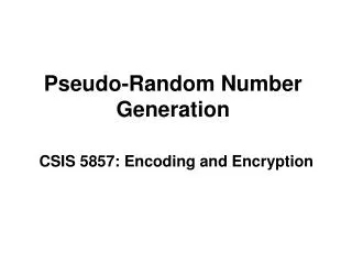
Pseudo-Random Number Generation • It is difficult to construct a truly random number generator. • Random number generators consist of a sequence of deterministically generated numbers that “look” random. • A deterministic sequence can never be truly random. • This property, though seemingly problematic, is actually desirable because it is possible to reproduce the results of an experiment! • Multiplicative Congruential Method xk+1=a xk modulo m • The constants a and m should follow the following criteria • For any initial seed x0, the resultant sequence should look like random • For any initial seed, the period (number of variables that can be generated before repetition) should be large. • The value can be computed efficiently on a digital computer.
Pseudo-Random Number Generation • To fit the above requirements, m should be chosen to be a large prime number. • Good choices for parameters are • m= 231-1 and a=75for 32-bit word machines • m= 235-1 and a=55for 36-bit word machines • Mixed Congruential Method xk+1 = (a xk + c) modulo m • A more general form: • where n is a positive constant • xk/m maps the random variates in the interval [0,1)
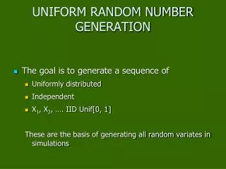
Quality of the Random Number Generator (RNG) • The random variate uk=xk/m should be uniformly distributed in the interval [0,1). • Divide the interval [0,1) into k subintervals and count the number of variates that fall within each interval. • Run the chi-square test. • The sequence of random variates should be uncorrelated • Define the auto-correlation coefficient with lag k > 0 Ckand verify that E[Ck] approached 0 for all k=1,2,… where uiis the random variate in the interval [0,1).
Some Probability Review/Results Pr{X=1}=p1 Pr{X=2}=p2 Pr{X=3}=p3 1 X 1 2 3 p1+ p2 + p3 p1+ p2 p1 X 1 2 3 • Probability mass functions • Cumulative mass functions
Some Probability Results/Review Probability density functions fX(x) x1 x 0 1 FX(x) x 0 • Cumulative distribution Pr{x=x1}= 0!
Independence of Random Variables Joint cumulative probability distribution. • Independent Random Variables. • For discrete variables • For continuous variables
Conditional Probability Conditional probability for two events. • Bayes’ Rule. • Total Probability
Expectation and Variance Expected value of a random variable • Expected value of a function of a random variable • Variance of a random variable
Covariance of two random variables The covariance between two random variables is defined as • The covariance between two independent random variables is 0 (why?)
Markov Inequality If the random variable X takes only non-negative values, then for any value a > 0. • Note that for any value 0<a < E[X], the above inequality says nothing!
Chebyshev’s Inequality If X is a random variable having mean μ and variance σ2, then for any value k > 0. x σ kσ kσ fX(x) μ • This may be a very conservative bound! • Note that for X~N(0,σ2), for k=2, from Chebyshev’s inequality Pr{.}<0.25, when in fact the actual value is Pr{.}< 0.05
The Law of Large Numbers Weak: Let X1, X2, … be a sequence of independent and identically distributed random variables having mean μ. Then, for any ε>0 • Strong: with probability 1,
The Central Limit Theorem Let X1, X2, …Xn be a sequence of independent random variables with mean μiand variance σι2. Then, define the random variable X, • Let • Then, the distribution of X approaches the normal distribution as n increases, and if Xi are continuous, then
Chi-Square Test • Let k be the number of subintervals, thus pi=1/k, i=1,…,k. • Let Ni be the number of samples in each subinterval. Note that E[Ni]=Npi where N is the total number of samples • Null HypothesisH0: The probability that the observed random variates are indeed uniformly distributed in (0,1). • Let T be • Define p-value= PH0{T>t} indicate the probability of observing a value t assuming H0 is correct. • For large N, T is approximated by a chi-square distribution with k-1 degrees of freedom, thus we can use this approximation to evaluate the p-value • The H0 is accepted if p-value is greater than 0.05 or 0.01
Monte-Carlo Approach to Evaluating Integrals Suppose that you want to estimate θ, however it is rather difficult to analytically evaluate the integral. • Suppose also that you don’t want to use numerical integration. • Let U be a uniformly distributed random variable in the interval [0,1) and ui are random variates of the same distribution. Consider the following estimator. Strong Law of Large Numbers • Also note that:
Monte-Carlo Approach to Evaluating Integrals Use Monte-Carlo simulation to estimate the following integral. • Let y=(x-a)/(b-a), then the integral becomes • What if • Use the substitution y= 1/(1+x), • What if
Example: Estimate the value of π. (-1,1) (1,1) (-1,-1) (1,-1) • Let X, Y, be independent random variables uniformly distributed in the interval [-1,1] • The probability that a point (X,Y) falls in the circle is given by • SOLUTION • Generate N pairs of uniformly distributed random variates (u1,u2) in the interval [0,1). • Transform them to become uniform over the interval [-1,1), using (2u1-1,2u2-1). • Form the ratio of the number of points that fall in the circle over N
Discrete Random Variates Suppose we would like to generate a sequence of discrete random variates according to a probability mass function 1 u X x Inverse Transform Method
Discrete Random Variate Algorithm (D-RNG-1) Algorithm D-RNG-1 Generate u=U(0,1) If u<p0, set X=x0, return; If u<p0+p1, set X=x1, return; … Set X=xn, return; • Recall the requirement for efficient implementation, thus the above search algorithm should be made as efficient as possible! • Example: Suppose that X{0,1,…,n} and p0= p1 =…= pn = 1/(n+1), then
Discrete Random Variate Algorithm D-RNG-1: Version 1 Generate u=U(0,1) If u<0.1, set X=x0, return; If u<0.3, set X=x1, return; If u<0.7, set X=x2, return; Set X=x3, return; More Efficient • Assume p0= 0.1, p1 = 0.2, p2 = 0.4, p3 = 0.3. What is an efficient RNG? • D-RNG-1: Version 2 • Generate u=U(0,1) • If u<0.4, set X=x2, return; • If u<0.7, set X=x3, return; • If u<0.9, set X=x1, return; • Set X=x0, return;
Geometric Random Variables Let p the probability of success and q=1-p the probability of failure, then X is the time of the first success with pmf • Using the previous discrete random variate algorithm, X=j if As a result:
Poisson and Binomial Distributions Poisson Distribution with rate λ. • Note: • Note: • The binomial distribution (n,p) gives the number of successes in n trials given that the probability of success is p.
Accept/Reject Method (D-RNG-AR) Suppose that we would like to generate random variates from a pmf {pj, j≥0} and we have an efficient way to generate variates from a pmf {qj, j≥0}. Let a constant c such that • In this case, use the following algorithm • D-RNG-AR: • Generate a random variate Y from pmf {qj, j≥0}. • Generate u=U(0,1) • If u< pY/(cqY), set X=Y and return; • Else repeat from Step 1.
Accept/Reject Method (D-RNG-AR) Show that the D-RNG-AR algorithm generates a random variate with the required pmf {pj, j≥0}. 1 pi/cqi qi Therefore
D-RNG-AR Example Determine an algorithm for generating random variates for a random variable that take values 1,2,..,10 with probabilities 0.11, 0.12, 0.09, 0.08, 0.12, 0.10, 0.09, 0.09, 0.10, 0.10 respectively. • D-RNG-1: • Generate u=U(0,1) • k=1; • while(u >cdf(k)) • k=k+1; • x(i)=k; • D-RNG-AR: • u1=U(0,1), u2=U(0,1) • Y=floor(10*u1 + 1); • while(u2 > p(Y)/c) • u1= U(0,1); u2=U(0,1); • Y=floor(10*rand + 1); • y(i)=Y;
The Composition Approach Let X1 have pmf {qj, j≥0} and X2 have pmf {rj, j≥0} and define • Suppose that we have an efficient way to generate variates from two pmfs {qj, j≥0} and {rj, j≥0} • Suppose that we would like to generate random variates for a random variable having pmf, a(0,1). • Algorithm D-RNG-C: • Generate u=U(0,1) • If u <= a generate X1 • Else generate X2
Continuous Random VariatesInverse Transform Method Suppose we would like to generate a sequence of continuous random variates having density function FX(x) Algorithm C-RNG-1: Let U be a random variable uniformly distributed in the interval (0,1). For any continuous distribution function, the random variate X is given by FX(x) 1 x u X
Example: Exponentially Distributed Random Variable Suppose we would like to generate a sequence of random variates having density function • Solution • Find the cumulative distribution • Let a uniformly distributed random variable u • Equivalently, since 1-u is also uniformly distributed in(0,1)
Convolution Techniques and the Erlang Distribution Suppose the random variable X is the sum of a number of independent identically distributed random variables • Algorithm C-RNG-Cv: • Generate Y1,…,Yn from the given distribution • X=Y1+Y2+…+Yn. • An example of such random variable is the Erlang with order n which is the sum of n iid exponential random variables with rate λ.
Accept/Reject Method (C-RNG-AR) Suppose that we would like to generate random variates from a pdf fX(x) and we have an efficient way to generate variates from a pdf gX(x). Let a constant c such that • In this case, use the following algorithm • C-RNG-AR: • Generate a random variate Y from density gX(x). • Generate u=U(0,1) • If u< fX(Y)/(cgX(Y)), set X=Y and return; • Else repeat from Step 1.
Accept/Reject Method (C-RNG-AR) The C-RNG-AR is similar to the D-RNG-AR algorithm except the comparison step where rather than comparing the two probabilities we compare the values of the density functions. • Theorem • The random variates generated by the Accept/Reject method have density fX(x). • The number of iterations of the algorithm that are needed is a geometric random variable with mean c • Note: The constant c is important since is implies the number of iterations needed before a number is accepted, therefore it is required that it is selected so that it has its minimum value.
C-RNG-AR Example Use the C-RNG-AR method to generate random variates X that are normally distributed with mean 0 and variance 1, N(0,1). • First consider the pdf of the absolute value of |X|. • We know how to generate exponentially distributed random variates Y with rate λ=1. • Determine c such that it is equal to the maximum of the ratio
C-RNG-AR Example • C-RNG-AR for N(0,1): • u1=U(0,1), u2=U(0,1); • Y= -log(u1); • while(u2 > exp(-0.5(Y-1)*(Y-1))) • u1= U(0,1); u2=U(0,1); • Y= -log(u1); • u3= U(0,1); • If u3 < 0.5 X=Y; • Else X= -Y; • Suppose we would like Z~N(μ,σ2), then
Generating a Homogeneous Poisson Processes A homogenous Poisson process is a sequence of points (events) where the inter-even times are exponentially distributed with rate λ(The Poisson process will be studied in detail during later classes) • Let ti denote the ith point of a Poisson process, then the algorithm for generating the first N points of the sequence {ti, i=1,2,…,N} is given by • Algorithm Poisson-λ: • k=0, t(k)=0; • While k<N • k= k+1; • Generate u=U(0,1) • t(k)= t(k-1) – log(u)/lambda; • Return t.
Generating a Non-Homogeneous Poisson Processes Suppose that the process is non-homogeneous i.e., the rate varies with time, i.e.,λ(t) ≤λ, for all t<T. • Let ti denote the ith point of a Poisson process, andτ the actual time, then the algorithm for generating the first N points of the sequence {ti, i=1,2,…,N} is given by • Algorithm Thinning Poisson-λ: • k=0, t(k)=0, tau= 0; • While k<N • Generate u1=U(0,1); • tau= tau – log(u1)/lambda; • Generate u2= U(0,1); • If(lambda(tau)\lambda < u2) • k= k+1, t(k)= tau; • Return t.
Generating a Non-Homogeneous Poisson Processes Again, suppose that the process is non-homogeneous i.e., the rate varies with time, i.e.,λ(t) ≤λ, for all t<T but now we would like to generate all points ti directly, without thinning. • Assuming that we are at point ti, then the question that we need to answer is what is the cdf of Si where Siis the time until the next event • Thus, to simulate this process, we start from t0 and generate S1 from FS1 to go to t1=t0+S1. Then, from t1, we generate S2 from FS2 to go to t2=t1+S2 and so on.
Example of Non-Homogeneous Poisson Processes Suppose that λ(t)= 1/(t+α), t≥0, for some positive constant a. Generate variates from this non-homogeneous Poisson process. • First, let us determine the rate of the cdf • Inverting this yields
Example of Non-Homogeneous Poisson Processes • Inverse Transform • Thus we start from t0=0 …
The Composition Approach • Suppose that we have an efficient way to generate variates from cdfs G1(x),…, Gn(x). • Suppose that we would like to generate random variates for a random variable having cdf • Algorithm C-RNG-C: • Generate u=U(0,1) • If u<p1, get X from G1(x), return; • If u<p1+p2, get X from G2(x), return; • …
Polar Method for Generating Normal Random Variates Y R θ X • Let X and Y be independent normally distributed random variables with zero mean and variance 1. Then the joint density function is given by • Then make a variable change • The new joint density function is Exponential with rate 1/2 Uniform in the interval [0,2π]
Polar Method for Generating Normal Random Variates Generates 2 independent RVs (-1,1) (1,1) (V1,V2) (-1,-1) (1,-1) • Algorithm C-RNG-N1: • Generate u1=U(0,1), u2=U(0,1); • R= -2*log(u1); W= 2*pi*u2; • X= sqrt(R) cos(W); Y= sqrt(R) sin(W); • But, sine and cosine evaluations are inefficient! • Algorithm C-RNG-N2: • Generate u1=U(0,1), u2=U(0,1); • Set V1= 2*u1-1, V2= 2*u2-1; • S=V1*V1+V2*V2; • If S > 1, Go to 1 • R= sqrt(-2*log(S)/S); • X= R*V1; • Y= R*V2;
Simulation of Discrete Event Systems STATE TIME EVENT CALENDAR e1 t1 Update Time t’=t1 Update State x’=f(x,e1) e2 t2 … Delete Infeasible Events Add New Feasible Events CLOCK STRUCTURE RNG INITIALIZE
Verification of a Simulation Program • Standard debugging techniques • Debug “modules” or subroutines • Create simple special cases, where you know what to expect as an output from each of the modules • Often choosing carefully the system parameters, the simulation model can be evaluated analytically. • Create a trace which keeps track of the state variables, the event list and other variables.