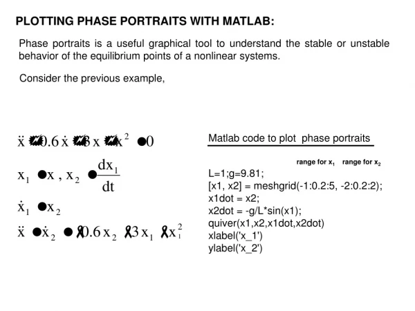
PLOTTING PHASE PORTRAITS WITH MATLAB:
120 likes | 157 Vues
Learn to plot phase portraits in Matlab to analyze system equilibrium points and stability, using the undamped simple pendulum as an example. Explore linearization techniques for nonlinear systems.

PLOTTING PHASE PORTRAITS WITH MATLAB:
E N D
Presentation Transcript
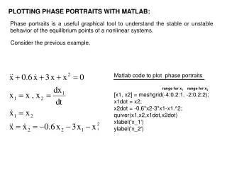
Matlab code to plot phase portraits L=1;g=9.81; [x1, x2] = meshgrid(-1:0.2:5, -2:0.2:2); x1dot = x2; x2dot = -g/L*sin(x1); quiver(x1,x2,x1dot,x2dot) xlabel('x_1') ylabel('x_2') range for x1 range for x2 PLOTTING PHASE PORTRAITS WITH MATLAB: Phase portraits is a useful graphical tool to understand the stable or unstable behavior of the equilibrium points of a nonlinear systems. Consider the previous example,
(-3,0) (0,0)
l g Matlab code to plot phase portraits θ Equilibrium points: (0, 0) and (p, 0) L=1;g=9.81; [x1, x2] = meshgrid(-1:0.2:5, -2:0.2:2); x1dot = x2; x2dot = -g/L*sin(x1); quiver(x1,x2,x1dot,x2dot) range for x1 range for x2 m Unstable Stable Example:Consider the undamped simple pendulum
(0,0) (p,0)
l e1 m For l=1 m At the equilibrium, all derivatives are zero Consider the small perturbations around the equilibrium point θd=0 Nonlinear terms can be linearized using the Maclaurin series.
m e1 l For θd=0 Higher order term clc;clear; A=[0 1;-9.81 0]; eig(A) ans = 0 + 3.1321i 0 - 3.1321i A Marginally stable For θd=p clc;clear; A=[0 1;9.81 0]; eig(A) ans = 3.1321 -3.1321 Unstable
Initial conditions Initial conditions [0.1;0] [0.1;0]
Example: Mathematical model of a nonlinear system is given by the equation Where f(t) is the input and x(t) is the output of the system. Find the equilibrium points for f=80 and linearize the system for small deviations from the equilibrium points. Find the response of the system The state variables are chosen as x1=x and x2=dx/dt=dx1/dt >>solve(‘64000*x1^2/(x1+2)=1.2’) x1d=0.00613, x2d=0 For the equilibrium condition x1=x1d+e1=0.00613+e1 x2=x2d+e2=e2
x1=x1d+e1=0.00613+e1 x2=x2d+e2=e2 f=fd+u
=0 =0 clc;clear; A=[0 1;-390.52 -9]; eig(A) ans = -4.5000 +19.2424i -4.5000 -19.2424i Stable system
Matlab code for step input with magnitude 2 clc;clear a=[0 1;-390.52 -9];b=[0 0.015]';c=[1 0];d=0; sys=ss(a,b,c,d); t=[0:.025:2]; [y,t,x]=step(sys*2,t); plot(t,y,'--','Linewidth',2);axis([0 2 0 0.00015]);grid; xlabel('time (sec)');ylabel('Y output');title('Step Response') c=[0 1]
u(t) 2 t e2 e2 e1 e1 u(t) 2 t We can obtain the same result using Simulink.