Download
1 / 45
450 likes | 668 Vues
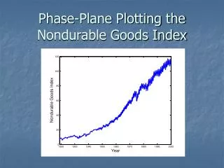
Phase-Plane Plotting the Nondurable Goods Index. Nondurable goods last less than two years: Food, clothing, cigarettes, alcohol, but not personal computers!! The nondurable goods manufacturing index is an indicator of the economics of everyday life.

E N D
Nondurable goods last less than two years: Food, clothing, cigarettes, alcohol, but not personal computers!! The nondurable goods manufacturing index is an indicator of the economics of everyday life. The index has been published monthly by the US Federal Reserve Board since 1919. It complements the durable goods manufacturing index.
What we want to do • Look at important events. • Examine the overall trend in the index. • Have a look at the annual or seasonal behavior of the index. • Understand how the seasonal behavior changes over the years and with specific events.
Events and Trends • Short term: • 1929 stock market crash • 1937 restriction of money supply • 1974 end of Vietnam war, OPEC oil crisis • Medium term: • Depression • World War II • Unusually rapid growth 1960-1974 • Unusually slow growth 1990 to present • Long term increase of 1.5% per year
The evolution of seasonal trend • We focus on the years 1948 to 1999 • We estimate long- and medium-term trend by spline smoothing, but with knots too far apart to capture seasonal trend • We subtract this smooth trend to leave only seasonal trend
Smoothing the data We want to represent the data yj by a smooth curve x(t). The curve should have at least two smooth derivatives. We use spline smoothing, penalizing the size of the 4th derivative. A function Pspline in S-PLUS is available by ftp from ego.psych.mcgill.ca/pub/ramsay/FDAfuns
Seasonal Trend • Typically three peaks per year • The largest is in the fall, peaking at the beginning of October • The low point is mid-December
Phase-Plane Plots • Looking at seasonal trend itself does not reveal as much as looking at the interplay between: • Velocity or its first derivative, reflecting kinetic energy in the system. • Acceleration or its second derivative, reflecting potential energy. • The phase-plane diagram plots acceleration against velocity. • For purely sinusoidal trend, the plot would be an ellipse.
Phase-plane plot for 1964 There are three large loops separated by two small loops or cusps: • Spring cycle: mid-January into April • Summer cycle: May through August • Fall cycle: October through December
1929 through 1931 • The stock market crash shows up as a large negative surge in velocity. • Subsequent years nearly lose the fall production cycle, as people tighten their belts and spend less at Christmas.
1937 and 1938 The Treasury Board, fearing that the economy was becoming overheated again, clamped down on the money supply. The effect was catastrophic, and nearly wiped out the fall cycle. This new crash was even more dramatic than that of 1929, but was forgotten because of the outbreak of World War II.
During World War II, the seasonal cycle became very small, since the war, and the production that fed it, lasted all year long. Now look at three pivotal years, 1974 to 1976, when the Vietnam War ended and the OPEC oil crisis happened. Watch the shrinking of the fall cycle.
These days Over the last ten years the size of all three cycles have become much smaller. Why? • Is variation now smoothed out by information technology? • Are the aging baby boomers spending less? • Are personal computers, video games, and other electronic goods really durable? • Has manufacturing now moved off shore?
Conclusions • We can separate long- and medium-term trends from seasonal trends by smoothing. • Phase-plane plots are great ways to inspect seasonality. • Derivatives were used in two ways: to penalize roughness, and to reflect the dynamics of manufacturing.
Trends in Seasonality We see by inspection that seasonal trends change systematically over time, and can also change abruptly. We first estimate the principal components of seasonal variation, using a version of principal components analysis adapted to functional data, and sensitive only to effects periodic over one year.
The Components • Relative sizes of spring and summer cycles (53%) • Joint size of spring and summer cycles (25%) • Size of fall cycle (11%)
Plotting Component Scores We can compute scores at each year for these three principal components, sometimes called empirical orthogonal functions. Plotting the evolution of these scores over the 51 years shows some interesting structural changes in the economics of everyday life.
Wrap-up • Phase-plane plots are good for inspecting seasonal quasi-harmonic trends • Principal components analysis reveals main components of variation in seasonal trend. • Plotting component scores shows how trend has evolved.
This was joint with work with James B. Ramsey, Dept. of Economics, New York University, and is reported in: Ramsay, J. O. and Ramsey, J. B. (2001) Functional data analysis of the dynamics of the monthly index of non‑durable goods production. Journal of Econometrics, 107, 327‑344.