Download
1 / 29
290 likes | 317 Vues
Explore various distribution simulation methods like Uniform, Normal, Exponential, and more with practical applications and generation techniques.

E N D
A Summary of Random Variable Simulation Ideas for Today and Tomorrow
Uniform • X is uniformly distributed on the interval [a,b] • We write X~unif(a,b) • Uses • the basis for generating all random variables • can be used as a model for a quantity that is known to vary between a and b for which little else is known
Uniform • method of generation • use a random number generator included in software or write your own generator to generate Y~unif(0,1) • set X=(b-a)Y+a
We write X~N( , ) Normal • X is normally distributed with mean and variance • Uses • model errors in various processes • quantities that are sums of lots of other quantities
set Normal • method of generation • generate Y~N(0,1) • Box-Muller method • Polar-Marsaglia method
If , let The Polar-Marsaglia Method Let U1 and U2 be independent unif(0,1) rv’s. Let V1=2U1-1 and V2=2U2-1. Then X1=CV1 and X2=CV2 are independent and normally distributed with mean 0 and variance 1.
X is exponentially distributed with rate • We write X~exp(rate= ) Exponential • Uses • lifetimes • waiting times • service times • interarrival times
invert the cdf Exponential • method of generation The inverse cdf method: • set X=F-1(U) where U~unif(0,1)
we write X~DE( , ) Double Exponential • X has a bilateral (double) exponential distribution with location parameter and shape parameter • as a “jump process” in finance
the pdf is • consider the case • this is a “back-to-back” exponential with rate • simulate Y~exp(rate= ) • flip a fair coin to add • shift X=Y+ Double Exponential • method of generation
We write Gamma • X has the gamma distribution with shape parameter and scale parameter • Uses • sum of exponential event times • time to complete a task consisting of consecutive exponential events
the pdf is • use accept-reject sampling to generate • set Gamma • method of generation
We write Weibull • X has the Weibull distribution with shape parameter and scale parameter • Uses • time to complete a task • time to equipment failure • differs from exponential in that failure probability can vary over time • used in reliability testing
the pdf is • the cdf is • invert Weibull • method of generation • set X=F-1(U)
We write Beta • X has the beta distribution with parameters and • Uses • well represents bounded rv’s with various kinds of skew (many shapes!) • distribution of random proportions • rough model in the absence of data
the pdf is • generate independently • set Beta • method of generation
we write Pareto • X has the Pareto distribution with parameter • Uses • modeling incomes • modeling stock price returns • monitoring production processes
the pdf is • the cdf is • invert Pareto • method of generation • set X=F-1(U)
we write Cauchy • X has the Cauchy distribution with location parameter and scale parameter • Uses • mostly interesting for theoretical reasons
let Cauchy • method of generation • the pdf is • simulate Y~Cauchy(0,1) by inverse cdf method
we write logistic • X has the logistic distribution with location parameter and scale parameter • Uses • growth models • logistic regression
the pdf is • the cdf is • invert: logistic • method of generation • set X=F-1(U)
we write • is the natural log of a Weibull with Gumbel • X has the Gumbel distribution with location parameter and scale parameter • Uses • modeling extreme events
invert the cdf • or, take the natural log of a Weibull generated with Gumbel • method of generation
Note: and are not the mean and variance! • ln(X) ~ N( , ) • time to perform a task, especially a very quick task (pdf spikes near 0 for small ) Log-Normal • We write X~LN( , ) • Uses • model quantities that are products of a large number of random quantities
generate Y~N( , ) • let Log-Normal • method of generation
so, we can count events occurring before 1 unit of time by where Yi are iid exponentials. Poisson • counts the number of events that occur in a unit of time when events are occurring at a constant rate • counts the number of events that occur in a unit of time when events are occuring with exponential inter-occurrence times
Note that if U~unif(0,1), • So, we also know that Poisson • Specifically, to generate a Poisson rv with rate ,we will generate exponential rate inter- arrival times.
Poisson • Let a=e-1, b=1, counter=0 • Algorithm: • Generate U~unif(0,1) and let b=bU • If b<a, done: return counter • otherwise, counter = counter+1