Download
1 / 102
1.04k likes | 1.3k Vues
Optimal Estimation of Bottom Friction Coefficient for Free-Surface Flow Models. Yan Ding, Ph.D. Research Assistant Professor, National Center for Computational Hydroscience and Engineering, The University of Mississippi, University, MS 38677.

E N D
Optimal Estimation of Bottom Friction Coefficient for Free-Surface Flow Models Yan Ding, Ph.D. Research Assistant Professor, National Center for Computational Hydroscience and Engineering, The University of Mississippi, University, MS 38677 Presentation for ENGR 691-73, Numerical Optimization, Summer Session, 2007- 2008
Introduction and Brief Review of Optimal Parameter Estimation Optimal Estimation of Manning’s Roughness Coefficient in Shallow Water Flows Variational Parameter Estimation of Manning’s Roughness Coefficient Using Adjoint Sensitivity Method Discussions Outline
I. Introduction and Brief Review of Optimal Parameter Estimation
Parameters in Mathematical Models • Physical Parameters: measurable describe physical properties and simple physical processes have state equations which describe the physical process, e.g., =(T, P) • Empirical Parameters: unmeasurable complicated physical processes, unmeasurable from the physical point of view, e.g., Manning Roughness n, without state equation have to be determined from historical observations
Complexity of Manning’s Roughness Physical-process-based parameters Depth (m) Bridge Pier Main Channel Flood Plain Manning Roughness n = f(surface friction, bed form friction, wave, flow unsteadiness ,vegetation (?), etc) [1] , or n=n(x,y) : distributed parameters, spatially dependent Moyie River at Eastport, Idaho
Objectives of Presentation • Theoretical Framework for estimation of the Manning’s roughness by using optimal theories (Optimization) • Estimate the Manning’s roughness so as to minimize the discrepancy between computation and observation • Compare the efficiency and accuracy of various minimization procedures(High Performance of Identification) • Demonstrate practical parameter estimation to determine the Manning’s roughness for the CCHE1D and CCHE2D hydrodynamic models (Application)
General Analysis Tools Based on Optimal Theories Trust Region Method
Ill-Posedness of the Problem of Parameter Estimation The inverse problem for parameter estimation is often ill-posed. This ill-posedness is characterized by: • Non-uniqueness (Identifiability) The concept of identifiability addresses the question whether it is at all possible to obtain unique solutions of the inverse problem for unknown parameters of interest in a mathematical model from data collected in the spatial and time domains • Instability of the identified parameters Instability here means that small errors in data will cause serious errors in the identified parameters
History of Parameter Identification in Computational Hydroscience and Engineering • 1980s- Sakawa and Shindo (1980): a general optimal control algorithm Bennett and McIntosh (1982) and Prevost and Salmon (1986) : early work of variational method for tidal flow Heemink (1987) : EKF to flow identification (English channel) Panchang and O’Brien (1989) : Adjoint parameter identification (API) for bottom friction in a tidal channel Das and Lardner (1990, 1992) : bottom friction in a tidal channel
History of Parameter Identification in Computational Hydroscience and Engineering • 1990s- Yu and O’Brien (1991) : wind stress coefficient Richardson and Panchang (1992) : API for eddy viscosity, Zhou et al (1993): LMQN for meteorology Kawahara and Goda (1993) : eddy viscosity by maximum likelihood Lardner and Song (1995): eddy viscosity profile in a 3-d channel Hayakawa and Kawahara (1996) : velocity and phase by Kalman filter Atanov et al (1999): Roughness in open channel (de St. Venant equation) Ding & Wang (2003): API for Manning’s roughness coefficient in channel network in the CCHE1D model Ding & Wang (2004): Sensitivity-equation method for estimation of spatially-distributed Manning’s n in shallow water flow models (CCHE2D)
Reviews and Books about Parameter Identification • Review Ghil and Malanotte-Rizzoli (1991), Advances in Geophysics, vol.33 : Review about data assimilation in meteorology and oceanography, Navon (1998), Dynamics of Atmosphere and Oceans, vol 27: Review about parameter identification, identifiability and nonuniqueness related to ill-poseness of parameter identification problem • Books: Malanotte-Rizzoli, P. (1996): Modern Approaches to Data Assimilation in Ocean Modelling, Elsevier Oceano. Series Wunsch, C. (1996): The Ocean Circulation Inverse Problem, Cambridge University Press. Nocedal & Wright (1999), Numerical Optimization, Springer, NY
Journals SIAM J. on Control and Optimization /Optimization (OOOOO) J. Acoust. Soc. (OOOO) J. Geophysical Research (OOOO) Water Resource Research (American Geophysical Union) (OOO) Monthly Weather Review (OOO) Tellus (OO) ASCE J. Hydr. Engrg. (OO) Web Resources SPIN Database Online( http://scitation.aip.org/jhtml/scitation/search/) American Institute of Physics, NY ISI Web of Science (http://scientific.thomson.com/products/wos/ ) EI (Engineering Village) http://daypass.engineeringvillage.com/ Journals and Online Resources about Optimal Parameter Estimation
To evaluate the discrepancy between computation and observation, one can define a weighted least squares form as Output Error Measure: Performance Function J or its discrete form: where X = physical variables, the weight W is related to confidence in the observation data. The superscript ‘obs’ means measured data. t0 : the starting time, tf : the final time during the period of parameter identification
Mathematical Framework for Optimal Parameter Estimation • The parameter identification is to find the parameter n satisfying a dynamic system such that • Local minimum theory[3] : Necessary Condition: If n* is the true value, then J(n*)=0; Sufficient Condition: If the Hessian matrix 2J(n*) is positive definite, then n*is a strict local minimizer of f subject to
Establish an Iterative Procedure to Search for Optimal Parameter Value: Sakawa-Shindo Method (1) • Assumed that the computational domain =l(l=1,2,..L) in which the Manning roughness is nk, by adding a penalty term, the performance function can be modified as the following form, where (k) is iteration step in the Sakawa-Shindo procedure, C(k) is a diagonal weighting matrix at the (k)th step, the weight matrix is renewed at every step. Fig. Spatially-distributed parameters
Sakawa-Shindo Procedure (2) • Correction Formulation ofnk Considering the first-order necessary condition J(n)=0, the parameter can be estimated from the previous value as follow, • Change the weighting matrix C(l) : • If J(k+1)J(k), then C(k+1)=0.9C(k),otherwise C(k)=2.0C(k), • continue to do next estimation of n.
Evaluate the gradient of performance function the sensitivity matrix can be computed by 1. Influence Coefficient Method[2] : Parameter perturbation trial-and-error 2. Sensitivity Equation Method: Forward computation Solve the sensitivity equations obtained by taking the partial derivatives with respect to each parameter in the governing equations and all of boundary conditions 3. Adjoint Equation Method: Backward computation The sensitivity is evaluated by the adjoint variables governed by the adjoint equations derived from the variational analysis. Sensitivity Analysis
Trust Region Methods: change searching directions and step size Sakawa-Shindo method[4] considering the first order derivative of performance function only, stable in most of practical problems Linear Search Approaches: directions are pre-determined, change step size Conjugate Gradient Methods (e.g. Fletcher-Reeves method) [5] The convergence direction of minimization is considered as the gradient of performance function. Truncated Newton Methods or Hessian-free Newton methods Limited-Memory Quasi-Newton Method (LMQN) [3] Newton-like method, applicable for large-scale computation, considering the second order derivative of performance function (the approximate Hessian matrix) Minimization Procedures for Unconstrained Optimization
Unconstrained optimization methods Step length Search direction 1) Line search 2) Trust-Region algorithms Searching in Parameter Space
Methods for Unconstrained Optimization 1) Steepest descent (Cauchy, 1847) 2) Newton 3) Quasi-Newton (Broyden, 1965; and many others)
Methods for Unconstrained Optimization (cont.) 4) Conjugate Gradient Methods (1952) is known as the conjugate gradient parameter 5) Truncated Newton method (Dembo, et al, 1982) 6) Trust Region methods
Step Length Computation 1) Armijo rule: 2) Goldstein rule:
3) Wolfe conditions: Implementations: Shanno (1978) Moré - Thuente (1992-1994)
Remarks: 1) The Newton method, the quasi-Newton or the limited memory quasi-Newton methods has the ability to accept unity step lengths along the iterations. 2) In conjugate gradient methods the step lengths may differ from 1 in a very unpredictable manner. They can be larger or smaller than 1 depending on how the problem is scaled*. *N. Andrei, (2007) Acceleration of conjugate gradient algorithms for unconstrained optimization. (submitted JOTA)
Given the iteration of a line search method for parameter n nk+1 = nk + kdk k = the step length of line search sufficient decrease and curvature conditions dk = the search direction (descent direction) Bk = nnsymmetric positive definite matrix For the Steepest Descent Method: Bk = I Newton’s Method: Bk= 2J(nk) Quasi-Newton Method: Bk= an approximation of the Hessian 2J(nk) Limited-Memory Quasi-Newton Method (LMQN) (Basic Concept 1)
Difficulties of Newton’s method in large-scale optimization problem: obtain the inverse Hessian matrix, because the Hessian is fully dense, or, the Hessian cannot be computed. BFGS (Broyden, Fletcher, Goldfarb, and Shanno, 1970) Constructs the inverse Hessian approximation , L-BFGS (One of LMQN method) (1) However, all of the vector pairs (sk, yk) have to be stored.
Updating process of the Hessian by using the information from the last m Q-N iterations L-BFGS (2) Where m is the number of Q-N updates supplied by the user, Generally [3] , 3 m 7 and Only m vector pairs (si, yi),i=1, m, need to be stored
Flow chart of parameter identification by using L-BFGS procedure
The purpose of the L-BFGS-B method is to minimize the performance function J(n) , i.e., min J(n), subject to the following simple bound constraint, nmin n nmax, where the vectors nmin and nmax mean lower and upper bounds on the Manning roughness. L-BFGS-B is an extension of the limited memory algorithm (L-BFGS) for unconstrained problem proposed in [6]. For the details about the limited memory algorithm for bound constrained optimization method, see [7]. L-BFGS-B
When the difference of the identified parameters is very large, the identification suffers from the poor scaling problem. lead to instability in the identification process Scaling : parameter transformation n/=Dn Gill et al [8] proposed the diagonal matrix D But we found this approach could not do very well, even destabilize the identification process (L-BFGS). Therefore, we proposed the two approaches for forming the matrix D Scaling Problems Scaling 1 Scaling 2
II. Optimal Estimation of Spatially-Distributed Manning’s Roughness Coefficient in Shallow Water Flows
Application to Shallow Water Equations • Governing Equations in , where n is the Manning roughness coefficient, is to be identified.
Given the boundary S=S1S2, the boundary conditions are subject to on S1, on S2, The initial conditions are at t=t0, Boundary and Initial Conditions
The sensitivity equations of sensitivity vector can be derived, by taking the partial derivative with respect to each parameter in the governing equations. Sensitivity Equations for Forward Computation
Boundary and Initial Conditions • Boundary Conditions • Initial Conditions This becomes a well-posed problem for the identification of Manning Roughness in shallow water flows
Numerical Techniques and Program Properties • Numerical method to solve the sensitivity equations: Efficient Element Method (CCHE2D) • Structural modules for parameter identification are compatible with CCHE2D; • The user can choose an appropriate minimization procedure (Sakawa-Shindo method, L-BFGS, or L-BFGS-B) (Multifunction) • Easy to prepare the input and control data files
Numerical Results (Verification) • Strategy for verification Initial Values of parameters : far from the true values Verify : identifiability, uniqueness of solution, stabilityof process
Observation Data and Identified Parameters(Open channel flow: N=3) (a) Longitudinal profile of water elevation (b) Velocity vectors and observed points
Cases for verification of parameter identification (Open channel flow) Number of Q-N updates in L-BFGS: m=5
Case 1 : Sakawa-Shindo Method (a) Iterations of Manning’s n (b) Iterations of performance function
Case 2 : L-BFGS Method (a) Iterations of Manning’s n (b) Iterations of performance function
Case 3 and Case 4: L-BFGS +Scaling (1) (a) L-BFGS+Scaling 1 (b) L-BFGS+Scaling 2
Case 3 and Case 4: L-BFGS +Scaling (2) Norm of error = ||n -nobj||2 (a) Comparison of J (b) Comparison of norm of error
Case 5 and Case 6: L-BFGS-B Excellent!! Bound constraint: 0.00001 n 1.0 (a) L-BFGS-B (b) L-BFGS-B+Transition
Summary of Verification for Open Channel Cases Remark: The L-BFGS-B with bound constraints has excellent features for stabilizing the identification process and accelerating the convergence.
Application: East Fork River n5 n4 Partition of Manning’s n L = 5 n3 n2 n1 Length of study reach = 3.3km