Transforming Relationships in Two-Variable Data Analysis
Explore transforming exponential growth into linear growth using logarithmic transformations, power law models, and cautionary notes on correlation, regression, and lurking variables in data analysis.

Transforming Relationships in Two-Variable Data Analysis
E N D
Presentation Transcript
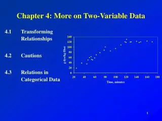
Chapter 4: More on Two-Variable Data 4.1 Transforming Relationships 4.2 Cautions 4.3 Relations in Categorical Data
Year 1990 1993 1994 1995 1996 1997 1998 1999 Cell Phone Users (thousands) 5,283 16,009 24,134 33,786 44,043 55,312 69,209 86,047 Example
What’s going on here? • Do the data (y) increase by a constant amount each year? • This would suggest a linear model. • Or, do the data increase by a fixed percentage each year? That is, can you multiply the y-value by a fixed number to get the next year’s number, and then multiply that number by the fixed number to get the following year’s number? • This would suggest an exponential model.
Transformation of the Variables • The next step is to apply a mathematical transformation that changes exponential growth into linear growth. • The transformation that can help here is to take the logarithm of the y-variable, then re-plot and re-calculate the LSR.
New LSR, with Transformed y Residuals Plot
We are dealing with a transformed y-value! • Model: • In order to use the model for prediction, we must “undo” the logarithm transformation to return to the original units of measurement. • How do we do this? • Now use the new model to predict cell phone subscribers for 2000.
Homework • Problem 4.6, p. 212 • Problem 4.11, p. 213 • Reading: pp. 203-215
Power Law Models • General form of a power law model: • Biologists have found that many characteristics of living things are described quite closely by power laws. • For example, the rate at which animals use energy goes up as the ¾ power of their body weight (Kleiber’s Law).
LSR and Power Law Models • As we saw in the last section, exponential growth models become linear when we apply the logarithm transformation to the response variable y. • Power law models become linear when we apply the logarithm transformation to both variables, x and y.
Log Transformations for Power Law Models • Looking carefully at the last equation, the power (p) becomes the slope of the straight line that links log y to log x. • We can estimate what power (p) the law involves by regressing log y on log x and using the slope of the regression line to estimate the power.
Problem 4.13, p. 219 Log of Both Variables
Undoing the Transformation • Let’s do the math to see what we need:
HW Problem: • 4.14, p. 220
Warm-Up Problem • 4.25, pp. 224-225 • Create appropriate model • Predict seed count for tree with seed weight of 1,000 mg.
4.25 I. II. Log of both L1 and L2 Axes off to see trend IV. III. Y2 vs. original data V.
4.2 Cautions about Correlationand Regression • The correlation (r) and the LSR line are not resistant. • As we have seen, extrapolation is often dangerous. • Predicting past the x-variable for which the model was developed.
The French Paradox • The paradox refers to the fact that the French have long had low rates of heart disease (Japan is the only developed country with a lower rate), despite a diet relatively rich in saturated animal fats. The French propensity to drink wine the way some Americans guzzle soft drinks has been cited as a likely explanation of the paradox, since numerous studies have indicated that alcohol consumed in moderation helps to prevent atherosclerosis, or accumulation of fatty deposits in arteries, which is the underlying cause of most heart attacks. + from NY Times article
Lurking Variables • As we discussed in the example of amount of wine consumed vs. number of incidents of heart disease, there can be other variables not measured in a correlation study that may influence the interpretation of relationships among those variables. • Lurking Variables • It is possible to show, for example, that there is a high correlation between shoe size and intelligence for a group of children varying in age from, say, 4 to 15. • What is the lurking variable? • To control for age, we can calculate the correlation between shoe size and IQ for each of the different ages. • Age 4, 5, 6, …
Correlation Between Shoe Size and IQ?(Common Response) Age IQ Shoe Size
Lurking Variables ThatChange Over Time • Many lurking variables change systematically over time. • One useful method for detecting lurking variables is to plot both the response variable and the regression residuals against the time order of the observations (whenever the time order is available). • See Example 4.12, p. 228
Using Averaged Data • Be careful when applying the results of a study that uses averages to individuals. • Problem 4.31, p. 231
Causation • Simply put, a strong correlation between two variables says nothing about one variable causing the other. One variable may in fact cause the other to change, but a correlation or LSR line cannot tell us that. • More investigation is needed! • A designed study with proper experimental controls should be used.
Figure 4.22, p. 232 • Causation • Common Response • Confounding
Confounding • The effects of two variables on a response variable are said to be confounded when they cannot be distinguished from one another. • Definition: Two or more variables that might have caused an effect were simultaneously present, so that we do not know to which to attribute the effect. • See 1, Example 4.13 (p. 232), and explanation, p. 233, top of p. 234. • Does this mean that we cannot ever suggest causation? • Read the two paragraphs on p. 235 (establishing causation).
Causation • Example 4.14, p. 232 • Numbers 1 and 2 (p. 233)
Common Response • Example 4.15, p. 233
Homework • Reading through p. 240
Problems • Problems on p. 237: • 4.33, 4.34, 4.35 • 4.73, p.257
Problem 4.73, p. 257 Power law model might best fit, so take log of L1 and L2. Plot below of L3 and L4.
4.73, cont. The pendulum period is proportional to the square root of its length.
4.3 Relations in Categorical Variables • There are many relationships of interest to us that cannot be described by using correlation and LSR techniques. • Recall that correlation and LSR require both variables to be quantitative. • Often, we want to study the relationship between two variables that are inherently categorical.
cell Two-Way Table (Ex. 4.19, p. 241)
Two-Way Table • The row variable is level of education. • In this study, is level of education the explanatory or response variable? • The column variable is age. • Explanatory or response? • Marginal distributions: • The distributions of education alone and age alone are called marginal distributions because their totals are in the margins: Education at the right, and age at the bottom.
Marginal Distributions • It is often advantageous to display the marginal distribution in percents instead of raw numbers.
Conditional Distributions • The previous graph looked at the breakdown of education levels for the entire population. Many times, however, we are looking for breakdowns (i.e., distributions) for a certain group within the population. • For example, of those people with 4+ years of college, look at the distribution across age groups. • Let’s complete a bar graph for this comparison. • This is a conditional distribution.
Different Question • What proportion of each age group received 4+ years of college education?
Problems • 4.53, p. 245 • 4.59, p. 251