Transforming Relationships in Bivariate Data: Techniques and Applications
This chapter delves into the intricacies of transforming relationships within bivariate data by exploring different methods such as logarithmic and power transformations. With a focus on real-world examples, such as the relationship between brain weight and body weight in animals, the text illustrates how transforming variables can clarify their relationships and enhance predictive accuracy. The chapter emphasizes the importance of selecting appropriate transformations to ensure linearity and improve data analysis, ultimately leading to more reliable predictions in various fields of study.


Transforming Relationships in Bivariate Data: Techniques and Applications
E N D
Presentation Transcript
4.1 Transforming Relationships • Animal’s Brain Weight vs. Weight of Body Outliers r=.86
Drop Outliers Logarithm r=.50
Plot Logarithm vs. Logarithm r=.96 The vertical spread about the LSRL is similar everywhere, so the predictions of brain weight from body weight will be pretty precise (high r2) – in LOG SCALE
Working with a function of our original measurements can greatly simplify statistical analysis. • Transforming- How?
Recall… • Chapter 1 we did Linear Transformations • Took a set of data and transformed it linearly • Called: SHIFTING C to F Meters to Miles
A Linear Transformation CANNOT make a curved relationship between 2 variables “straight” • Resort to common non-linear functions like the logarithm, positive & negative powers • We can transform either one of the explanatory/response variables OR BOTH • when we do we will call the variable “t”
Real World Example: We measure fuel consumption of a car in miles per gallon Engineers measure it in gallons per mile (how many gallons of fuel the car needs to travel 1 mile) Reciprocal Transformation: 1/f(t) My Car- 25 miles per gallon 1/25=.04 gallons per mile
Monotonic Function • A monotonic function f(t) moves in one direction as its argument “t” increases • Monotonic Increasing • Monotonic Decreasing
Monotonic Increasing: a + bt slope b>0 Positive “t”
Monotonic Decreasing: a + bt slope b<0 Positive “t”
Nonlinear monotonic transformations change data enough to change form or relations between 2 variables, yet preserve order and allow recovery of original data.
Strategy: • If the variable that you want to transform has values that are 0 or negative apply linear transformation (add a constant) to get all positive. • Choose power or logarithmic transformation that approximately straightens the scatterplot.
Ladder of Power Transformations: Power Function: tP
Power Functions: • Monotonic Power Function For t > 0…. 1. Positive p – are monotonic increasing 2. Negative p – are monotonic decreasing
Monotonic Decreasing- Hard to interpret because reversed order of original data point • We want to make all tP therefore monotonic increasing. We can apply a LINEAR TRANSFORMATION
This is a line This is log t
Concavity of Power Functions: P is greater than 1 = - Push out right tail & pull in left tail - Gets stronger as power p moves up away from 1 P is less than 1 = - Push out left tail & pull in right tail - Gets stronger as power p moves down away from 1
P= Use
How do you know what transformation will make the scatterplot straight? ** DO NOT just push buttons!! ** • We will develop methods of selection 1. Logarithmic Transformation 2. Power Transformation
Exponential Growth A variable grows… Linearly: Exponentially:
The King’s Chess Board… King’s Offer: 1,000,000 grains - 30 days Wise Man: 1 grain per day and double for 30 days
Suspect Exponential Growth… • Calculate Ratios of Consecutive Terms - IF approximately the same… continue
Suspect Exponential Growth… 2. Apply a Transformation that: a. Transforms exponential growth into linear growth b. Transforms non-exponential growth into non-linear growth
Logarithm Review… • log(AB)= • log(A/B)= • logXp =
The Transformation… We hypothesize an exponential model of the form y=abx To gain linearity, use the (x, log(y)) transformation Form? –
When our data is growing exponentially… if we plot the log of y versus x, we should observe a straight line for the transformed data!
LOG (Y) = -263 + 0.134 (year) R-sq = 98.2%
LOG (New Y) = -189 + 0.0970(New X) R-sq = 99.99%
Predictions in Exponential Growth Model • Regression is often used for predictions • In exponential growth, ________ rather than actual values follow a linear pattern • To make a prediction of Exp. Growth we must thus “undo” the logarithmic transformation. • The inverse operation of a logarithm is _____________________
LOG (New Y) = -189 + 0.0970(New X) R-sq = 99.99% Predict the number of cell phone users in 2000.
If a variable grows exponentially… its ___________ grow linearly! In other words… if (x, y) is exponential, then (x, log(y)) is linear!
Power Law Model Example: Pizza Shop- order pizza by diameter 10 inch 12 inch 14 inch Amount you get depends on the area of the pizza Area circle = pi times the square of the radius Power Law Model
Power Laws • We expect area to go up with the square of dimension • We expect volume to go up with the cube of a dimension Real Examples: Many Characteristics of Living Things Kleiber’s Law- The rate at which animals use energy goes up as the ¾ power of their body weight (works from bacteria to whales).
Power Laws Become Linear • Exponential growth becomes linear when we apply the logarithm to the response variable (y). • Power Laws become linear when we apply the logarithm transformation to BOTH variables.
To Achieve Linearity… • The power law model is • Take the logarithm of both sides of equation (this straightens scatterplot) • Power p in the power law becomes the slope of the straight line that links log(y) to log(x) • Undo transformation to make prediction
Fish Example… Read Example 4.9 page 216 Model: weight = a x length3
Log (weight) = log a + [3x log(length)] • Yes appears very linear- perform LSRL on [log(length), log(weight)]