Download
1 / 36
360 likes | 518 Vues
The Physics of High Speed Logic. An account of the lessons learnt when assembling systems using Schottky TTL in the 1970s. Agenda. History understanding the interconnect Two worlds analogue and digital The interconnect a path of no return Distributing power

E N D
The Physics of High Speed Logic An account of the lessons learnt when assembling systems using Schottky TTL in the 1970s
Agenda • History • understanding the interconnect • Two worlds • analogue and digital • The interconnect • a path of no return • Distributing power • the ‘decoupling’ capacitor
Oliver Heaviside 1850-1925 In 1868 Heaviside went to Denmark and became a telegrapher. He progressed quickly in his profession and returned to England in 1871 to take up a post in Newcastle upon Tyne in the office of Great Northern Telegraph Company which dealt with overseas traffic.
Heaviside and E/M Theory While still working as chief operator in Newcastle he began to publish papers on electricity, the first in 1872 and then the second in 1873 was of sufficient interest to Maxwell that he mentioned the results in the second edition of his Treatise on Electricity and Magnetism.
The Victorian Internet • Submarine cables 1000’s of km in length. • Transit time around 5 ms/km • Pulses with a risetime of ms. • So risetime was less than transit time and true pulse (transmission line) behaviour was observed. • Heaviside discussed may of the practical situations which arose including the passage of pulses through one another when travelling in opposite directions in a transmission line.
Kilkenny Cats • "There once was two cats of Kilkenny Each cat thought there was one cat too many So they fought and they fit And they scratched and they bit 'Til instead of two cats there weren't any."
Wireless The invention and exploitation of radio communication moved the focus from the pulse to the sinusoidal wave.
Wireless Connection • Information is transferred at a slow rate compared to the frequency of the carrier wave. • One could think of transmitter and receiver being connected by the carrier wave. • In principle the transmitter was aware of the receiver’s existence.
The Digital Revolution • The introduction of pulsed RF in radar during WW2 heralded the return of digital technology. • Computers developed in the 50’s and 60’s were increasingly digital. • The slow speeds of the early computers (pulse risetimes >> transit times) meant that designers could still think in analogue terms. • The high impedances of valves (around 100kohms) meant that the environment through which the signals travelled was essentially capacitative.
The Digital Revolution 1970 – present • A move from sine wave to pulse • A move from high to low impedance • A move from slow rate of information transfer to fast 100k > Z > 100 Ω risetime < propagation delay
930 Series Diode-Transistor Logic Three-Input NAND Gate • Note that transistors were feeble (10mA collector current), so 6k load resistance. • Incidentally, why drive from the collector?
Stray Capacitance When transistor turns off, C charges through 6k resistor. Let C = 10pF (about 10-20cm length); RC = 60ns. C
Something had to be done - TTL By adding the top transistor, current could now be forced into the stray capacitance reducing the risetime. Incidentally, transistors were now getting more beefy. stray capacitance
Schottky TTL • This was the final improvement (?). Schottky clamping kept the transistors out of saturation and speeded up switching times. We now had a 1 ns switching edge with 4.5 volt swing and the ability to drive stray capacitance.
What No-one Noticed • Was that the shorter risetimes and ability to switch lower impedances meant that the interconnect was now behaving as a transmission line. • Now a transmission line appears to the driver as a resistive load; it does not require push-pull driving. • An open collector, better still, an open emitter is all that is required.
Emitter Coupled Logic • If ZL = Z0 there will be no reflections. • ECL was rejected as a logic family because of its inability to drive stray capacitance. • The whole point was that it didn’t need to: it needed to drive resistance!
Path of No Return • Once our systems are operating in the transmission line universe we cannot ignore the return path. • Because the transmission line ‘crept up’ on digital designers they built unreliable systems where return paths were frequently remote from signal lines. • Manufacturers guidance onten included the injunction to ‘avoid earth loops’. Clearly the direct consequence of this is to eliminate return path connections.
‘Decoupling’ Capacitor A typical use of a decoupling capacitor would be in a valve circuit where C decouples the anode supply from signals caused by variations of the supply voltage. C 0V
..and • This idea of a capacitor ‘shorting’ the AC signal provided the paradigm for the understanding of decoupling in logic systems.
Decoupling in Logic • An analogue engineer would probably view the capacitors as ‘shorting out’ the noise on the power rails. • The problem was that he did not know the source impedance of the noise and hence could only guess at the appropriate value of C. C C
A better approach … • .. is to think of C as a charge reservoir which provides the local current peak as the gates switch and prevents the rail voltage dropping before reinforcements of electrons arrive from further along the power supply chain. • Now we can do some calculations. • If we have a 16 output device with each pin driving a 100 Ω impedance interconnect, we get a peak current of approaching 1A. • If we can allow the rail to drop by a max of 0.25V before help arrives in, say, 10ns, we need a capacitor of around 40nF.
Tantalum beads • Tantalum beads come in right capacities and working voltages and are physically small.
Are capacitors inductive? • The engineer had an additional problem: • He was told that the high frequencies involved required a high frequency capacitor. • This would mean that it should be used below its self-resonant frequency. • This means something like a silvered mica component which are only available in relatively low values. • The engineer was even threatened with the possibility that the wrong type of capacitor could ‘blow up’!
In addition … • .. the engineer was told that the stray inductance of the larger capacitor would negate its decoupling ability. • After all, above its self resonant frequency it is behaving like an inductor, not a capacitor, and you want a capacitor.
http://ecmweb.com/content/protecting-dc-fed-electronic-equipmenthttp://ecmweb.com/content/protecting-dc-fed-electronic-equipment
.. A thought .. • I was discussing this with Ivor one day when he said something like, ‘Look, when you buy a big capacitor you get a small one free’. Free with every large capacitor
In other words • You do not experience the total lumped inductance of the component when you address it with a step current demand. • The step propagates into the capacitor sending charge out as it propagates inwards. • It was a small step from here to view the capacitor as a transmission line:
The capacitor is a transmission line • This was the moment when the world changed. • If the capacitor is simply conductors distributed in space then the very idea of a capacitor disappears. • On a practical note, we will never see the total lumped inductance of a capacitor when we address it with a step. • In fact, the bigger the capacitor, the less effect the current step will have and the less ‘noise’ will be generated.
Stray Inductance • Before we leave inductance, though, we need to return to the power distribution systems to consider the role of stray inductance in the interconnections. • The loop shown in blue represents the current path from the reservoir capacitor to the package. • By making reasonable assumptions about its dimensions we can calculate a value of around 30 nH. C
The effect of stray indictance • If we take our previous value for ΔI = 1A and .. • We assume the transient risetime is 1 ns (note this is now the signal risetime and not the 10ns previously assumed for the time for additional charge to arrive from the power supply). • We get: • E = L ΔI/Δt = 30 volts !! • Clearly such a high value of stray inductance is unacceptable and would cause the power supply to the device to collapse for a short time.
The geometry • Can we improve this? • Incidentally, note that the standard pinout is worst case, maximising the stray inductance.
Yes we can! I have a sample of a two layer board designed on this basis. 0V +5V
Lessons for Today • The fallacy of linearity. • Technology does not proceed in a linear fashion. The next obvious step may be incorrect. There are times when a fundamental rethink is required. • The application of science. • Do not be afraid to return to first principles. • Be ready to enjoy being surprised. • You might be like Alice who spotted a white rabbit with a pocket watch and followed it to discover a new world.
Noise • EMC
EMC Would the blue line represent safety?