Probabilistic models
Explore deterministic and hierarchical Bayesian models, Gibbs sampling, and Bayesian belief nets for inference and modeling relationships in data. Learn practical approaches and strategies to harness the power of probabilistic modeling.


Probabilistic models
E N D
Presentation Transcript
Probabilistic models Jouni Tuomisto THL
Outline • Deterministic models with probabilistic parameters • Hierarchical Bayesian models • Bayesian belief nets
Deterministic models with probabilistic parameters • Inputs are uncertain, but causal relations are assumed certain. • Works well with established situations, especially if physical foundations. • Exposure = ∑ (ci ti) / ∑ ti • i = microenvironment • c = concentration • t = time
Functional vs. probabilistic dependency Va1=2.54*Ch1^2 Va2=normal(2.54*Ch1^2,2)
Hierarchical Bayesian models • Relations are probabilistic • Gibbs Sampler • Another MCMC (Markov chain Monte Carlo) Method • Update a single parameter at a time • Sample from conditional distribution • When other parameters are fixed
Gibbs sampling • To introduce the Gibbs sampler, consider a bivariate random variable (x; y), and suppose we wish to compute one or both marginals, p(x) and p(y). • The idea behind the sampler is that it is far easier to consider a sequence of conditional distributions, p(x |y) and p(y |x), than it is to obtain the marginal by integration of the joint density p(x; y), e.g., • p(x) = ∫ p(x; y)dy.
Gibbs sampling in practice • The sampler starts with some initial value y0 for y and obtains x0 by generating a random variable from the conditional distribution p(x |y = y0). • The sampler then uses x0 to generate a new value of y1, drawing from the conditional distribution based on the value x0, p(y j x = x0). The sampler proceeds as follows • xi ≈p(x |y = yi-1) (proportionality) • yi ≈p(y |x = xi) • Repeating this process k times, generates a Gibbs sequence of length k, where a subset of points (xj; yj) for 1 ≤j ≤m < k are taken as our simulated draws from the full joint distribution.
Hierarchical model with parameters and hyperparameters • A useful graphical tool for representing hierarchical Bayes models is the directed acyclic graph, or DAG. In this diagram, the likelihood function is represented as the root of the graph; each prior is represented as a separate node pointing to the node that depends on it.
Bayesian belief nets • Relations are described either with conditional probabilities P(x|y), P(y) or marginal probabilities P(x), P(y) and a rank correlation between them. • You need to get the conditional probabilities from somewhere. • Unlike hierarchical Bayes model, belief nets are not developed for updating when new data comes out. • The model is used to make inference.
Bayesian belief nets P(rain) P(sprinkler | rain) P(grass wet | sprinkler, rain)
Uninet: diagram view • V1: rain (mm/day) • V2: sprinkler on (h/day) • V3 ”wetness” of grass (range 0-1)