Spectral Analysis in Time Series: Insights and Applications
260 likes | 332 Vues
Explore spectral analysis, Fourier representation, and spectral density functions for understanding periodicities in time series data. Learn about frequency limits, aliasing, and applications in various fields of data analysis.

Spectral Analysis in Time Series: Insights and Applications
E N D
Presentation Transcript
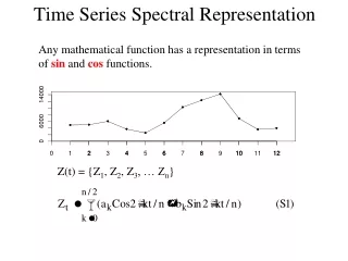
Time Series Spectral Representation Any mathematical function has a representation in terms of sin and cos functions. Z(t) = {Z1, Z2, Z3, … Zn}
Spectral Analysis • Represent a time series in terms of the wavelengths associated with oscillations, rather than individual data values • The spectral density function describes the distribution of these wavelengths • Spectral analysis involves estimating the spectral density function. • Fourier analysis involves representing a function as a sum of sin and cos terms and is the basis for spectral analysis
Why Spectral Analysis • Yields insight regarding hidden periodicities and time scales involved • Provides the capability for more general simulation via sampling from the spectrum • Supports analytic representation of linear system response through its connection to the convolution integral • Is widely used in many fields of data analysis
Frequency and Wavenumber cycles/time radians/time Due to orthogonality of Sin and Cos functions
Frequency Limits Lowest frequency resolved Highest frequency resolved, corresponds to n/2 (Nyquist frequency) General case, time interval ∆t
Aliasing Due to discretization, a sparsely sampled high frequency process may be erroneously attributed to a lower frequency
Equivalent complex number representation Note: Integer truncation is used in the sum limits. For example if n=5 (odd) the limits are -2, 2. If n=6 (even) the limits are -2, 3. (Same number of fourier coefficients as data points) Complex conjugate pair
Fourier representation of an infinite (non periodic) discrete series Discrete transform pair Lowest frequency Highest frequency Spacing As
Fourier representation of an infinite (non periodic) discrete series Discrete transform pair Re-center on [(-n-1)/2, (n-1)/2] for
Fourier transforms for discrete function on infinite domain (aperiodic) Wei section 10.5
Fourier transforms for continuous function on finite domain (periodic) Wei section 10.6.1
Fourier transforms for continuous function on infinite domain (aperiodic) Wei section 10.6.2
Frequency domain representation of a random process • Z(t) and C(w) are alternative equivalent representations of the data • If Z(t) is a random process C(w) is also random • ACF(Z(t))≡Spectral density function(C(w))
Spectral representation of a stationary random process Autocorrelation Autocorrelation function Time Series Fourier Transform Fourier Transform Spectral density function Fourier coefficients Smoothing
Time Domain Frequency Domain C1, C2, C3, … Z1, Z2, Z3, …
|Ck|2 is random because Zt is random Decomposition of variance Power at low frequency Persistence indicated by ACF The Periodogram |Ck|2 k/n Wei section 12.1
Time Domain r=0.9 r=0.2
Frequency Domain r=0.9 r=0.2
The Spectral Density Function The spectral density function is defined as S(w)dw=E(|C(w)|2) Wei section 12.2, 12.3
Problem Estimating S(w) • Z(t) Stationary C(w) Independent • |C(w)|2 has 2 degrees of freedom (from real and imaginary parts • More data ∆w gets smaller, but still 2 degrees of freedom n=200 n=50
S(w) estimated by smoothing the periodogram • Balance Spectral resolution versus precision • Tapering to minimize leakage to adjacent frequencies • Confidence bounds by 2 based on number of degrees of freedom involved with smoothing • Multitaper methods • A lot of lore
Spectral analysis gives us • Decomposition of process into dominant frequencies • Diagnosis and detection of periodicities and repeatable patterns • Capability to, through sampling from the spectrum, simulate a process with any S(w) and hence any Cov() • By comparison of input and output spectra infer aspects of the process based on which frequencies are attenuated and which propagate through