Download
1 / 65
680 likes | 1.05k Vues
The Spectral Representation of Stationary Time Series. Stationary time series satisfy the properties: Constant mean ( E ( x t ) = m ) Constant variance (Var( x t ) = s 2 ) Correlation between two observations ( x t , x t + h ) dependent only on the distance h.

E N D
Stationary time series satisfy the properties: • Constant mean (E(xt) = m) • Constant variance (Var(xt) = s2) • Correlation between two observations (xt, xt + h) dependent only on the distance h. • These properties ensure the periodic nature of a stationary time series
Recall and X1, X1, … , Xk and Y1, Y2, … , Yk are independent independent random variables with is a stationary Time series where l1, l2, … lk are k values in (0,p)
We can give it a non-zero mean, m, by adding mto the equation With this time series and
We now try to extend this example to a wider class of time series which turns out to be the complete set of weakly stationary time series. In this case the collection of frequencies may even vary over a continuous range of frequencies [0,p].
The Riemann integral The Riemann-Stiltjes integral If F is continuous with derivative f then: If F is is a step function with jumps pi at xi then:
First, we are going to develop the concept of integration with respect to a stochastic process. Let {U(l): l[0,p]} denote a stochastic process with mean 0 and independent increments; that is E{[U(l2) - U(l1)][U(l4) - U(l3)]} = 0 for 0 ≤ l1 < l2 ≤ l3 < l4 ≤ p. and E[U(l) ] = 0 for 0 ≤ l ≤ p.
In addition let G(l) =E[U2(l) ] for 0 ≤ l ≤ p and assume G(0) = 0. It is easy to show that G(l) is monotonically non decreasing. i.e. G(l1) ≤ G(l2) for l1 < l2 .
Now let us define: analogous to the Riemann-Stieltjes integral
Let 0 = l0 < l1 < l2 < ... < ln = p be any partition of the interval. Let . Let lidenote any value in the interval [li-1,li] Consider: Suppose that and there exists a random variable V such that *
Let {X(l): l [0,p]} and {Y(l): l [0,p]} denote a uncorrelated stochastic process with mean 0 and independent increments. Also let F(l) =E[X2(l) ] =E[Y2(l) ] for 0 ≤ l≤ p and F(0) = 0. Now define the time series {xt : tT}as follows:
Thus the time series {xt : tT} defined as follows: is a stationary time series with: F(l) is called the spectral distribution function: If f(l) = Fˊ(l) is called then is called the spectral density function:
Note The spectral distribution function, F(l), and spectral density function, f(l) describe how the variance of xt is distributed over the frequencies in the interval [0,p]
The autocovariance function, s(h), can be computed from the spectral density function, f(l), as follows: Also the spectral density function, f(l), can be computed from the autocovariance function, s(h), as follows:
Example: Let {ut : tT} be identically distributed and uncorrelated with mean zero (a white noise series). Thus and
Example: Suppose X1, X1, … , Xk and Y1, Y2, … , Yk are independent independent random variables with Let l1, l2, … lk denote k values in (0,p) Then
If we define {X(l): l[0,p]} and {Y(l): l[0,p]} Note:X(l) and Y(l) are “random” step functions and F(l) is a step function.
Another important comment In the case when F(l) is continuous then
Sometimes the spectral density function, f(l), is extended to the interval [-p,p] and is assumed symmetric about 0 (i.e. fs(l) = fs(-l) = f(l)/2 ) in this case It can be shown that
From now on we will use the symmetric spectral density function and let it be denoted by, f(l). Hence
Let {xt : tT} be any time series and suppose that the time series {yt : t T} is constructed as follows: : The time series {yt : t T} is said to be constructed from {xt : t T} by means of a Linear Filter. Linear Filter as output yt input xt
Let sx(h) denote the autocovariance function of {xt : tT} and sy(h) the autocovariance function of {yt : t T}. Assume also that E[xt] = E[yt] = 0. Then: :
Hence where of the linear filter
Note: hence
Let a0 =1, a1, a2, … aq denote q + 1 numbers. Spectral density function Moving Average Time series of order q, MA(q) Let {ut|t T} denote a white noise time series with variance s2. Let {xt|t T} denote a MA(q) time series with m = 0. Note: {xt|t T} is obtained from {ut|t T} by a linear filter.
Now Hence
Let b1, b2, … bp denote p + 1 numbers. Spectral density function Autoregressive Time series of order p, AR(p) Let {ut|t T} denote a white noise time series with variance s2. Let {xt|t T} denote a AR(p) time series with d = 0. Note: {ut|t T} is obtained from {xt|t T} by a linear filter.
Now Hence
Autocorrelation function and partial autocorrelation function