Download
1 / 7
70 likes | 231 Vues
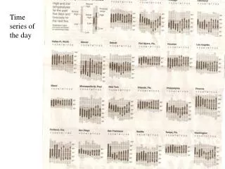
Time series of the day. Stat 153 - 11 Sept 2008 D. R. Brillinger Simple descriptive techniques. Trend X t = + t + t. Filtering y t = r=-q s a r x t-r Simple moving average s = q , a r = 1/(2q+1) Filters may be in series. Differencing

E N D
Stat 153 - 11 Sept 2008 D. R. Brillinger Simple descriptive techniques Trend Xt = + t + t Filtering yt = r=-qs ar xt-r Simple moving average s = q , ar = 1/(2q+1) Filters may be in series
Differencing yt = xt - xt-1 = xt "removes" linear trend Seasonal variation model Xt = mt + St + t St St-s 12 xt = xt - xt-12 , t in months
Stationary case, autocorrelation estimate at lag k, rk t=1N-k (xt- )(xt+k - ) over t=1N (xt - )2 autocovariance estimate at lag k, ck t=1N-k (xt - )(xt+k - ) / N
Departures from assumptions Nonstationarity Trend - OLS Seasonality - trig functions Outliers Missing values