Download
1 / 34
340 likes | 356 Vues
Analogue and digital techniques in closed loop regulation applications. Digital systems • Sampling of analogue signals • Sample-and-hold • Parseval’s theorem. Sampling process. T. Continuous Function f(t). Series of samples. Sampler (t). Reconstruction ?.

E N D
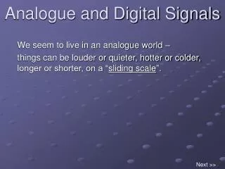
Analogue and digital techniques in closed loop regulation applications Digital systems • Sampling of analogue signals • Sample-and-hold • Parseval’s theorem
Sampling process T Continuous Function f(t) Series of samples Sampler (t) Reconstruction ?
From time domain to frequency domain Fourier transform y(t) is a real function of time We define the Fourier transform Y(f) A complex function in frequency domain f Y(f) is the spectral or harmonic representation of y(t) Frequency spectrum
Y(f) From time domain to frequency domain Example of Fourier transform y(t) t -T T Real even functions
From time domain to frequency domain NB: Comments on unit with Fourier function Use of =2f instead of f
Linear System b() Fourier series Fourier transform Fourier series
T T = Complex Fourier Coefficients Periodic function f(t) a series of frequencies multiple of 1/T
Principle To be minimal
Analysis in frequency domain • F()= Fourier transform of f(t) • ()= Fourier transform of (t) • F’()= Fourier transform of f’(t) Convolution in the frequency domain
n=-1 n=0 n=1 0 Analysis of () Periodic function Decomposition in Fourier series
Transform of f’(t) Convolution
Aliasing 0 Primary components Fundamental components Complementary components Complementary components The spectra are overlapping (Folding) Folding frequency
highest frequency component Requirements for sampling frequency • The sampling frequency should be at least twice as large as the highest frequency component contained in the continuous signal being sampled • In practice several times since physical signals found in the real world contain components covering a wide frequency range •NB:If the continuous signal and its n derivatives are sampled at the same rate then the sampling time may be:
Window Can we reconstruct f(t) ? f’(t) f °(t) f(t) Sampler Filter In the frequency domain
Back to time domain Convolution Window in the time domain f’(t) in the time domain
Reconstruction f(t) t nT (n+1)T (n+2)T (n+3)T Interpolation functions
Analogue and digital techniques in closed loop regulation applications Zero-order-hold
Reconstruction of sampled data To reconstruct the data we have a series of data Approximation A device which uses only the first term f[kT] is called a Zero-order extrapolator or zero-order-hold
Source Sample-and-Hold devices
Sample-and-hold circuit Droop Input signal t Output signal Hold mode Hold mode Sample mode = Settling time = Acquisition time = Aperture time
F(s) Impulse response F(s)=L[h(t)] h(t) (t) t t k=0 Transfer function
Convolution f’=0 y(t)y*(t) Parseval’s theorem x(t) and y(t) have Fourier transform X(f) and Y(f) respectively
x(t)y(t) This expression suggests that the energy of a signal Is distributed in time with a density Or is distributed in frequency with density Parseval’s theorem
Thank you for your attention