Design Techniques for Analog Circuitry in High Energy Physics
This document outlines analog circuit design principles with a focus on active components in modern integrated circuit (IC) technologies. It covers essential topics like the basics of amplifiers, differential amplifiers, operational transconductance amplifiers (OTA), and preamplifier designs specifically tailored for high-energy physics applications. Key aspects related to amplifier stability, gain, and signal bandwidth are discussed, along with examples relevant to detector front-end applications. This guide serves as a fundamental resource for engineers working with analog circuits in a physics context.

Design Techniques for Analog Circuitry in High Energy Physics
E N D
Presentation Transcript
ANALOGUE CIRCUITSTECHNIQUES Part I April 16th , 2002 F. ANGHINOLFI CERN Francis.Anghinolfi@cern.ch F. A. CERN/EP
Outline From “active” components available in modern IC technologies, to the examples of amplifiers design used for High Energy Physics applications • 1- Introduction to analogue circuit • 2- Active elements in Integrated Circuit • 3- The bipolar transistor F. A. CERN/EP
Outline • 4- Basic of amplifier • 5- Differential amplifier • 6- OTA • 7- Two-stage differential amplifier • 8- Other amplifiers circuits • 9- Cascode circuits • 10- Charge Preamplifier • 11- Transimpedance Preamplifier • 12- Preamplifiers conclusions F. A. CERN/EP
1- Introduction to analogue circuit We will NOT talk about : • A lot of different circuit configurations used for applications in HEP, or outside of HEP (broadband telecommunications, HF, audio, etc …) • A lot of parameters which may widely influence a final circuit design (like DC operating point, offsets, internal noise sources, sensitivities to external sources, components non-uniformities, etc …) We will MAINLY talk about : • Some major aspects of linear amplifier design : building blocks, amplifier stability, amplifier gain, signal bandwidth • Two examples of signal amplifiers circuits developed for detector front-end F. A. CERN/EP
1- Introduction to analogue circuit REFERENCES: books IC technology “Physics in Semiconductor Devices” S. M. Sze, Wiley Amplifier design “Analog Integrated Circuits” Paul. R. Gray, Robert. G. Meyer, Wiley Detector Amplifier design “Low-Noise Wide-band Amplifiers in Bipolar and CMOS technologies” Z. Y. Chang, Willy M.C. Sansen, Kluwer Academic Publishers http http://www.prenhall.com/howe3/microelectronics/ F. A. CERN/EP
Vdd R Id Vout Vin Gnd 1- Introduction to analogue circuit Vdd Analog circuit Digital circuit P Id Vout N Vin Gnd Vout=f(Vin) Vin and Vout can take any value between Vdd and Gnd Vin=Gnd (0) or Vdd (1) Vout = Vdd(1) or Gnd(0) NON LINEAR SYSTEM LINEAR SYSTEM F. A. CERN/EP
threshold threshold 1- Introduction to analogue circuit Analog circuit Digital circuit Highly non linear High noise immunity* Immune to power supply variations* Carries only one bit of information Highly linear Sensitive to noise (… pickup, crosstalk …) Sensitive to power supplies Carries n bits of information ** ** = function of max. signal range versus noise level * = up to certain limits ! F. A. CERN/EP
Ic IB 2- Active Components in Integrated Circuit MOS TRANSISTOR BIPOLAR TRANSISTOR Surface effect conduction under the control of the gate potential Volume effect conduction under the control of the junctions potential Id Vg N npn IE F. A. CERN/EP
2- Active Components in Integrated Circuit MOS TRANSISTOR BIPOLAR TRANSISTOR W/L=transistor aspect ratio Only “fundamental” quantities (k= Boltzman constant, T= Temp., q= electron charge) Ko=f(mobility, gate capacitance, T, …) Vt=f(dopant, gate capacitance, fixed charges, …) F. A. CERN/EP
3- The Bipolar Transistor FIRST SOLID STATE TRANSISTOR (1947) BARDEEN, BRATTAIN AND SHOCKLEY F. A. CERN/EP
3- The Bipolar Transistor p-n junction A pn-junction in Silicon is the abutment of two Si volumes with free carriers of opposite polarities • Majority carriers diffuse from regions of high to regions of low concentration • An electric potential is created, which counteracts the diffusion current (drift current) • In equilibrium there is no net flow of carriers in the diode N P f Holes (+) Electrons (-) Depletion region F. A. CERN/EP
3- The Bipolar Transistor p-n junction Al SiO 2 Cathode Anode n+ p-substrate Depletion region Diffusion Anode Drift e h n+ + + + + + fo - - - - - e p Cathode h F. A. CERN/EP
3- The Bipolar Transistor p-n junction • Under zero bias there is a built-in potential across the junction • The built-in potential is: F. A. CERN/EP
3- The Bipolar Transistor p-n junction • For V>T (forward bias) • For V<0 (reversed bias) F. A. CERN/EP
3- The Bipolar Transistor E C p n n B Minority carriers (electrons diffusion into the base) No Bias Barrier is lowered : more electrons (min. carriers) diffuse to the base, may reach the opposite junction, and contribute to the current of the reverse_biased BC junction B-E maj. carriers flow (holes) Bias applied Base-Emitter Junction is forward biased Collector-Base Junction is reverse biased F. A. CERN/EP
3- The Bipolar Transistor E C p n n B e e h e h h n p n 0 + ++ Base-Emitter Junction is forward biased Collector-Base Junction is reverse biased F. A. CERN/EP
3- The Bipolar Transistor Conduction mechanism in a bipolar transistor is made of the MINORITY CARRIERS flowing through the base region Currents are flowing through semiconductors junctions, within the crystalline structure. Not a surface effect. F. A. CERN/EP
3- The Bipolar Transistor A B E C p n n B Higher « reverse » current in reverse biased Collector-Base Junction Forward biased Base-Emitter Junction No Bias Bias applied F. A. CERN/EP
3- The Bipolar Transistor Why is bipolar effect an « amplifying » device ? • Currents in junctions A and B are almost equal. • B-E junction (A) is forward biased (low impedance) • C-E junction (B) is reverse biased (high impedance) The collector node being high impedance (current source). It can be loaded with large resistors Rhigh The output power is Rhigh.I2 The emitter node is low impedance. The power at emitter node is Rlow.I2 The output power (at collector) is higher than the input power (at emitter) F. A. CERN/EP
3- The Bipolar Transistor Minority carriers concentration at x=0 (diffusion carrier density equation) Np0 is theintrinsec minority carrier concentration in the base and K is the boltzmann constant q the electron charge T is temperature = 26mV at 300K F. A. CERN/EP
3- The Bipolar Transistor The collector current is the result of the minority carrier concentration in the base crossing the B-E junction due to the electrial field direction A is cross section of the emitter Dn is the diffusion constant for electrons (the minority carriers in NPN device) With the equation of np(0) np0 is theintrinsec minority carrier concentration in the base F. A. CERN/EP
3- The Bipolar Transistor The base current IB is the result of two current (holes in case of NPN) contributions (namely diffusion current in emitter and recombination current within the base): Both IC and IB depend on the same term : The ratio Ic/Ib is called « forward current gain » : F. A. CERN/EP
Ic IB 3- The Bipolar Transistor b, the current gain between collector and base : By maximizing NA/ND ratio,and minimizing WB, the base width, it is possible to reach values of b=50-200 npn IE Transconductance : F. A. CERN/EP
Ic IB npn IE 3- The Bipolar Transistor VCE Exp. Increase Ic vs. VCE Characterisitc Small signal model ic (DIc) gm.vbe vbe Zi Zo (DVbe) (note : in all transparencies, explicit “-” sign is ignored) F. A. CERN/EP
Reminder : The MOS Transistor Id Vgs N Power 2 Increase Id vs. Vds Characteristics Small signal model id (DId) gm.vgs vgs Zi Zo (DVgs) F. A. CERN/EP
Linear models for Bipolar or MOS Transistor Small signal model i (DI) gm.v v Zi Zo (DV) For most linear applications, both MOS or bipolar are represented by similar model elements Values inside the model are different : F. A. CERN/EP
4- Basic of amplifier The simplest amplification circuit Vcc R Ic The collector of the npn transistor behaves as a current source : delivery of current “Ic” from a high impedance node IB Vo npn IE Vbe The voltage gain is given by Vo variation vs. Vbe variation Gnd F. A. CERN/EP
4 - Basic of amplifier The voltage gain is given by Vo variation vs. Vbe variation Vcc R Ic IB Vo npn IE Vbe Gnd F. A. CERN/EP
4 - Basic of amplifier The voltage gain is given by Vo variation vs. Vbe variation Vcc R Is called the transconductance ‘gm’ Ic IB npn Vo IE Vbe Gnd F. A. CERN/EP
4 - Basic of amplifier Vcc Typical values : R Ic IB Vo npn IE Vbe Gnd F. A. CERN/EP
4 - Basic of amplifier Vcc ic npn Can be represented by a “small-signal model” R vbe Ic ic (DIc) IB Vo npn gm.vbe vbe Ri Ro IE Vbe (DVbe) Gnd Ri, Ro represent the input and output impedances of the non-ideal transistor F. A. CERN/EP
Gm.vbe vbe vo Ri Ro//Z (DVo) (DVbe) 4 - Basic of amplifier Vcc “small-signal model” Z Ic IB Vo npn IE Vbe Gnd Ri, Ro represent the input and output impedances of the non-ideal transistor F. A. CERN/EP
4 - Basic of amplifier A very simple Gain-Bandwidth calculation model Vcc Gm.vbe vbe vo Ri (DVo) R C (DVbe) Ro R C Ic Usually Ro (output impedance of transistor) is much higher than R. The output stage has one single pole created by the resistive load (which defines gain) and the capacitive load. IB Vo npn IE Vbe Gnd F. A. CERN/EP
4 - Basic of amplifier Vcc R C The circuit gain at low frequency is : gm.R (as expected) The circuit transfer function has one pole at t =RC The circuit bandwidth limit (Gain >1) is at : Ic IB Vo npn IE Vbe Gnd F. A. CERN/EP
4 - Basic of amplifier Vcc Gain (vo/vi) dB Gm.R1 R C Gm.R2 Ic IB Vo npn 1/t 0 IE 1/R1.C 1/R2.C 1/tc Vbe (log scale) Gnd The maximum bandwidth of gain circuit with one pole is given by the input device transconductance and capacitive load. Example : gm = 10-2, C=1pF, tc=100ps, fc=1.6GHz F. A. CERN/EP
Vdd R Id Vo Vgs Gnd 4 - Basic of amplifier The simplest amplification circuit with a MOS transistor instead of a bipolar one. The drain of the MOS transistor behaves as a current source : delivery of current “Id” from a high impedance node The voltage gain is given by Vo variation vs. Vgs variation F. A. CERN/EP
Vdd R Id Vo Vgs Gnd 4 - Basic of amplifier The voltage gain is given by Vo variation vs. Vgs variation “gm” transconductance of MOS device F. A. CERN/EP
Vdd R Id Vo Vgs Gnd 4 - Basic of amplifier The voltage gain is given by Vo variation vs. Vgs variation F. A. CERN/EP
Vdd R Id Vo Vgs Gnd 4 - Basic of amplifier Typical values for modern MOS technology: F. A. CERN/EP
4 - Basic of amplifier VARIANT WITH “ACTIVE LOAD” Vdd The resistor load can be replaced by a transistor working as a current source. The high output impedance (drain of PMOS) is used as the load. Vbias P R=rds Id Small signal model Vo N vgs=0 ids Vgs P gm.vgs vgs rds vds Gnd Transconductance factor Output Impedance F. A. CERN/EP
4 - Basic of amplifier VARIANT WITH “ACTIVE LOAD” Ids ids D gm.vgs vgs rds S Transconductance factor Output Impedance Dids/Dvds is small - Equivalent output resistance is high (usually 50K to 1Mohms) Vds F. A. CERN/EP
4 - Basic of amplifier VARIANT WITH “ACTIVE LOAD” Vdd Vbias P R=rdsP gm.vgs rdsP vgs rdsN Id Vo N Transconductance factor Output Impedance Vgs Gnd and rds is usually large (>50K-1M ohms). Gain G reaches ~100 (40dB) F. A. CERN/EP
Vdd R Id Vo Vgs Gnd 4 - Basic of amplifier SINGLE-ENDED STRUCTURE • Output is sensitive to Vdd/Gnd fluctuation (poor Power Supply Rejection) • Output DC is related to input DC levels (no Common Mode Rejection) F. A. CERN/EP
R Id1 5- Differential Amplifier Vdd Because of the weaknesses of the single-ended structure (common-mode and power supply sensitivity), the differential amplifier is usually a preferred structure R Id2 Vo1 Vo2 Vi1 Vi2 2*Id Vc Gnd F. A. CERN/EP
R Id1 5 - Differential Amplifier Formulate : Vdd Vid is the differential signal at input Vcm the input signal common mode Vc the voltage to transistor source R Id2 From MOS transistor equations : Vo1 Vo2 Vi1 Vi2 2*Id Vc Gnd F. A. CERN/EP
Vdd R R Id1 Id2 Vo1 Vo2 Vi- Vi+ 2*Id Vc Gnd 5 - Differential Amplifier Differential Gain : Vid is the differential signal at input Vcm the input signal common mode Vc the voltage to transistor source Small signal Formulation, diff. Input variation : F. A. CERN/EP
Vdd R R Id1 Id2 Vo1 Vo2 Vi- Vi+ 2*Id Vc Gnd 5 - Differential Amplifier Vid is the differential signal at input Vcm the input signal common mode Vc the voltage to transistor source Is the input transistors transconductance We end up with the differential gain expressed as : F. A. CERN/EP
Vdd R R Id1 Id2 Vo1 Vo2 Vi- Vi+ 2*Id Vc Gnd 5 - Differential Amplifier Common Mode Gain : Vid is the differential signal at input Vcm the input signal common mode Vc the voltage to transistor source Small signal Formulation, Common Mode Input variation : If the tail current source is perfect (very high Z) : Vo outputs are insensitive to common mode input F. A. CERN/EP
R Id1 5 - Differential Amplifier Common Mode Gain : Vid is the differential signal at input Vcm the input signal common mode Vc the voltage to transistor source If the tail current source has impedance Rss Vdd R This is the common mode gain, which is much less than the differential gain, approx. by the factor R/(2Rss). Id2 Vo1 Vo2 Vi- Vi+ The ratio of the differential gain to the common mode gain, is called the Common Mode Rejection Ratio (CMRR). In our case : Rss 2*Id Gnd (CMRR easily reaches 1000 (60db)) F. A. CERN/EP
By similar reasoning, it can be shown that the differential structure can provide : • High Common Mode Rejection • High Power Supply Rejection Vdd R R Id1 Id2 Vo1 Vo2 • The other features are : • Differential gain formulation as for single-ended • Constant power consumption Vi- Vi+ 2*Id Vc Gnd 5 - Differential Amplifier F. A. CERN/EP