Download
1 / 35
350 likes | 489 Vues
Quantitative Precipitation Forecasting at the Hydrometeorological Prediction Center (HPC) www.hpc.ncep.noaa.gov. Dan Petersen HPC Forecast Operations Branch Dan.Petersen@noaa.gov (301)763-8201.

E N D
Quantitative Precipitation Forecasting at the Hydrometeorological Prediction Center (HPC) www.hpc.ncep.noaa.gov Dan Petersen HPC Forecast Operations Branch Dan.Petersen@noaa.gov (301)763-8201
Quantitative Precipitation Forecasting at the Hydrometeorological Prediction Center (HPC)Goals of Presentation • Short Range QPF Methods • Short Range QPF Case Study • Verification
Composing a QPF • Short range ( <12 hours ) • Forecast composed by blending the latest radar and satellite data with an analysis of Moisture/Lift/Instability and model output • Long range ( >12 hours ) • Forecast increasingly relies on model output of QPF, Moisture/Lift/Instability • Adjustments are made for known model biases and latest model trends/verification/comparisons (including ensembles)
Composing a QPF ( <12 hours) • Radar • Looping can show areas of training and propagation • Review radar-estimated amounts-Be wary of beam blocking, bright bands, overshooting tops & attenuation • Compare observations to estimates (Z – R relationship impact) • Satellite • Rainfall estimates from NESDIS/Satellite Analysis Branch • Looping images can show areas of training/development • Derived Precipitable Water, Lifted Indices, soundings, etc.
OH Valley Case Study-Using Models/Radar/Satellite to Compose QPF GFS 18z-00z QPF June 14 2005 from 12z Run
OH Valley Case Study-Using Models/Radar/Satellite to Compose QPFNAM 18z-00z QPF June 14 2005 from 12z Run
OH Valley Case Study-Using Models/Radar/Satellite to Compose QPFHPC Forecast qpf 18z-00z QPF Jun14-15 2005
OH Valley Case Study-Using Models/Radar/Satellite to Compose QPFNAM Forecast CAPE/CIN 18z June14 2005
OH Valley Case Study-Using Models/Radar/Satellite to Compose QPFNAM Forecast Precipitable Water 18z June14 2005
OH Valley Case Study-Using Models/Radar/Satellite to Compose QPFNAM Forecast Best Lifted Indices 18z June14 2005
OH Valley Case Study-Using Models/Radar/Satellite to Compose QPFNAM Forecast Boundary Layer Moisture Convergence 18z June14 2005 (none over OH River)
OH Valley Case Study-Using Models/Radar/Satellite to Compose QPF 1719z Radar June 14 2005
OH Valley Case Study-Using Models/Radar/Satellite to Compose QPF 1724z Satellite June 14 2005
Real Time Case Study-Short term QPFSatellite Derived Convective Available Potential Energy- June 14 2005 16z
Real Time Case Study-Short term QPFSatellite Derived Lifted Index June 14 2005 16z
Real Time Case Study-Short term QPFSatellite Derived Convective Inhibition June 14 2005 16z
Real Time Case Study-Short term QPFSatellite Derived Precipitable Water June 14 2005 16z
OH Valley Case Study-Short term QPFJune 14 2005 Storm Total Precipitation
OH Valley Case Study-Short term QPFObserved 06 hour amounts ending 00z June 15 2005
Case Study Results • NAM model diagnostics supported developing convection, but did not identify boundary to provide lift • Satellite derived products supported model prognostics favorable for convection plus (combined with radar) identified boundaries to provide lift
Verification-How much Improvement Can We Derive from Satellite/Radar/Model diagnostics?
Short Term QPF Benefits from Multi-sensor Analysis • Improved real time multi-sensor analysis would • Reduce uncertainty of real time satellite/radar estimates • Reduce uncertainty of post-event rainfall and time spent on quality control (more reliable verification) • Lead to improvements in moisture/lift/instability-related diagnostics/prognostics, and thus confidence in qpf and excessive rainfall forecasts • Questions/needed clarifications?
Composing a QPF • Must have knowledge of: • Climatology • Precipitation producing processes • Sources of lift (boundaries, topography too) • Forecasting Motion (propagation component vs. advection) • Identifying areas of moisture/lift/instability
Analysis (Synoptic/Mesoscale) • Perform a synoptic & mesoscale analysis • Upper air • Upper fronts, cold pools, jet streaks • Surface Data • Boundaries • Satellite Data • Moisture plumes, Upper jet streaks • Radar • Boundaries • Try to link ongoing precipitation with diagnostics
Analysis (Moisture) • Precipitable Water (PW) • Surface through 700 mb dew points • Mean layer RH • K indices • Loops of WV imagery/derived PWs • Consider changes in moisture • Upslope/Down slope • Veritical/Horizontal advection • Soil moisture • Nearby large bodies of water
Analysis (Lift) • Low/Mid level convergence • Lows, fronts, troughs • Synoptic scale lift • Isentropic • QG components (differential PVA & WAA) • Jet dynamics • Nose of LLJ • Left front/right rear quadrants of relatively straight upper jets with good along stream variation of speed • Mesoscale boundaries • Outflow, terrain, sea breeze • Orographic lift • Solar heating
Analysis (Instability) • Soundings are your best tool • CAPE/CIN is better than any single index • Beware!! Models forecast CAPE/CIN poorly • Equilibrium Level • Convective Instability • Mid-level drying over low-level moisture • Increasing low-level moisture under mid-level dry air • Changing Instability • Try to anticipate change from • Low level heating • Horizontal/Vertical temperature/moisture advection • Vertical Motion
Precipitation Efficiency Factors • Highest efficiency in deep warm layer • Rainfall intensity is greater if depth of warm layer from LCL to 0o isotherm is 3-4 km • Low cloud base • Collision-Coalescence processes are enhanced by increased residence time in cloud • Need a broad spectrum of cloud droplet sizes • present from long trajectories over oceans • Highest efficiency in weak to moderately sheared environments • Some inflowing water vapor passes through without condensing • Of the water vapor that does condense • Some evaporates • Some falls as precipitation • Some is carried (blown) downstream as clouds or precipitation • In deep convection, most of the water vapor input condenses
Low Level Jet • Nocturnal maximum in the plains • Inertial oscillation enhances the jet • Often develops in response to lee low development • LLJ can be enhanced by upper level jet streak • Barrier jets (near mountains) can play a role in focusing lift • Convection can induce very focused LLJs
LLJ Importance • Speed convergence max at nose of LLJ • Confluent flow along axis of the LLJ • Vertical/Horizontal Moisture Flux positively related to strength of LLJ • Differential moisture/temperature advection can lead to rapid destabilization • Quasi-Stationary LLJ can lead to cell regeneration/training • Often located on the SW flank of a backward propagating MCS
Movement of a system is dependent on cell movement and propagation • The vector describing the propagation is the vector anti-parallel to the LLJ Vprop = -VLLJ • The vector that describes the movement of the most active part of an MCS is represented by • V = Vcell + Vprop • Propagation is dependent on how fast new cells form along some flank of the system
Factors leading to training/regenerating convection • Slow moving low level boundary • Quasi-stationary low level jet • Quasi-stationary area of upper level divergence • Low level boundary (moisture/convergence) nearly parallel to the mean flow • Lack of strong vertical wind shear (speed & directional)