Download
1 / 31
330 likes | 553 Vues
Lecture, Summer Term 2013. Physics of the Atmosphere 2 Radiation and Energy Balance. Ulrich Foelsche Institute of Physics, Institute for Geophysics, Astrophysics, and Meteorology (IGAM) University of Graz und Wegener Center for Climate and Global Change ulrich.foelsche@uni-graz.at

E N D
Lecture, Summer Term 2013 Physics of the Atmosphere 2 Radiation and Energy Balance Ulrich FoelscheInstitute of Physics, Institute for Geophysics, Astrophysics, and Meteorology (IGAM)University of Grazund Wegener Center for Climate and Global Change ulrich.foelsche@uni-graz.at http://www.uni-graz.at/~foelsche/
Atmo II 01 Textbooks C. DonaldAhrens, Meteorology Today: An Introduction to Weather, Climate, and the Environment, Brooks/Cole, 9. Ed., ISBN: 0495555746 (also paperback) UB-Semesterhandapparat, IGAM-Library K.N.Liou, (Ed.), An Introduction to Atmospheric Radiation, Academic Press, 2nd Ed., ISBN: 978-0-12-451451-5, 2002 <http://books.google.at/books?id=mQ1DiDpX34UC> (partial) Murry L.Salby, Physics of the Atmosphere and Climate, Cambridge Univ. Press, 2nd Ed., ISBN: 978-0-521-76718-7, 2012 <http://books.google.at/books?id=CeMdwj7J48QC> (partial)
Atmo II 02 Lehrbücher Helmut Kraus, Die Atmosphäre der Erde - Eine Einführung in die Meteorologie, Springer, Berlin, 3. Auflage, ISBN: 978-3-540-20656-9 (auch paperback) UB-Semesterhandapparat, IGAM-Bibliothek Gösta H. Liljequist & Konrad Cehak, Allgemeine Meteorologie, Springer, Berlin, 3. Auflage ISBN: 3540415653 (nützliches deutsch-englisches Register) UB-Semesterhandapparat, IGAM-Bibliothek Ludwig Bergmann & Clemens Schaefer, Lehrbuch der Experimentalphysik, Band 7, Erde und Planeten, (Kapitel 3 – Meteorologie, Kapitel 4 – Klimatologie), de Gruyter, Berlin, ISBN: 978-3-11-016837-2 UB-Semesterhandapparat, IGAM-Bibliothek
Atmo II 03 Exams No, it will be the other way round – you will be forced to answer questions – in my office & IGAM Exam dates and registration via UNIGRAZonline: online.uni-graz.at Picture credit: Gary Larson
Atmo II 04 Different Aspects of Atmospheric Radiation UF
Atmo II 05 Physics of the Atmosphere II (1) Electromagnetic Waves NASA
Atmo II 06 The Electromagnetic Field Basic Properties of the Electromagnetic Field Within the framework of classical electrodynamic theory, it is represented by the vector fields: Electric fieldE [V/m] Magnetic fieldB [Vs/m2] = [T] (Tesla) To describe the effect of the field on material objects, it is necessary to introduce a second set of vectors: the Electric current densityj [A/m2] Electric displacement fieldD [As/m2] Magnetizing fieldH [A/m] The space and time derivativesof the vectors field are related by Maxwell's equations – we will focus on the differential form.
The magnetic fieldB and the magnetizing field H are related by where µ0 is the magnetic constant4π·10-7 VsA-1m-1 (exact), and M is the magnetic polarization – the mean magnetic dipole moment per volume. Atmo II 07 The Electromagnetic Field The electric fieldE and the electric displacement field D are related by where ε0 is the electric constant8.854187817·10-12 AsV-1m-1 (exact) [NIST Reference: http://physics.nist.gov/cuu/Constants/index.html], and P is the electric polarization – the mean electric dipole moment per volume.
The Second Maxwell Equation or Gauss’s Law for Magnetism: states that there are no magnetic charges (magnetic monopoles). The magnetic field has nosourcesorsinks – its field lines can only form closed loops. Atmo II 08 Maxwell's Equations in Matter The First Maxwell Equation, also known as Gauss’s Law: relates the divergence of the displacement field to the (scalar) free charge density: Positive electric charges are sources of the displacement field (negative electric charges are sinks). Closed field lines can be caused by induction.
The Fourth Maxwell Equation: shows that magnetic (magnetizing) fields can be caused by electric currents (Ampère’s Law), but also by changing electric (displacement) fields (Maxwell’s Correction – which is very important, since it “allows” for electromagnetic waves – also in vacuum). Atmo II 09 Maxwell's Equations in Matter The Third Maxwell Equation, or Faraday’s Law of Induction: describes how a time-varying magnetic field causes an electric field (induction).
Atmo II 10 Maxwell's Equations in Gas The previous formulations are known as Maxwell’s Macroscopic Equations or Maxwell’s Equations in Matter. Under specific conditions the relations on slide 07 can be simplified. The Earth's atmosphere is a linear medium– the induced polarization P is a linear function of the imposed electric field E. The Earth’s atmosphere is also an isotropic medium –P is parallel to E: The electric susceptibilityχe degenerates to a simple scalar (in general it would be a tensor of second rank) and we get: where ε is the permittivity (or dielectric constant in a homogenous medium) and εr = 1 + χe is the dimensionless relative permittivity, which depends on the material and is unity for vacuum.
Atmo II 11 Maxwell's Equations in Gas Similar considerations for M and H yield: where χm is the (scalar) magnetic susceptibility (in general it would be again a tensor of second rank), µ is the permeability and µr = 1 + χm is the dimensionless relative permeability (which is also unity in vacuum). The electric current density j is related to the electric field E via the electric conductivity σ [Ω-1m-1] (a scalar for isotropic media, but in general again a tensor) through the differential form of Ohm’s Law:
Atmo II 12 Maxwell's Equations in Neutral Gas The lower atmosphere (troposphere and stratosphere, at least up to ~ 50 km) is a neutral (ρfree = 0), and isotropic medium, and has a negligible electric conductivity (σ = 0) yielding j = 0. Maxwell’s equations can therefore be written as:
Atmo II 13 Electromagnetic Waves Maxwell's equations relate the vector fields by means of simultaneous differential equations. On elimination we can obtain differential equations, which each of the vectors must separately satisfy. Applying the curl operator on Faraday’s law, interchanging the order of differentiation with respect to space and time (which can be done for a slowly varying medium like the atmosphere is one at frequencies of practical interest) and inserting the fourth Maxwell equation yields: with we get
Atmo II 14 Electromagnetic Waves These partial differential equations are standard wave equations. Considering plane waves, the solutions have the form: where k is the wave number vector, pointing in the direction of wave propagation. The angular frequency, ω [rad/s] and the angular wave number, k [rad/m], are defined as (with k = |k|): and where ν is the frequency (Hz) and λis the wavelength [m]. Inserting the above solutions into Maxwell’s equations yields:
Atmo II 15 Electromagnetic Waves which shows that the field vectors E and B are perpendicular to each other and that both are perpendicular to k. Electromagnetic waves are thus transverse waves. micro.magnet.fsu.edu wikimedia
Atmo II 16 Electromagnetic Waves Inserting the first equation of slide 14 in to the wave equation using the vector identity: and the orthogonality yields With the definition of the phase velocity: we see that monochromatic electromagnetic waves propagate in a medium with the phase velocity:
Atmo II 17 Electromagnetic Waves And in vacuum we get: C0 = 299 792 458 m s-1 which is nothing else than the speed of light in vacuum In geometric optics the refractive index of a medium (n) is defined as the ratio of the speed of light in vacuum (c0) to that in the medium (c): which is known as the Maxwell Relation. In the Earth’s atmosphere the relative permeability is almost exactly = 1, thus we get (in a general, frequency-dependent form):
Atmo II 18 Electromagnetic Waves James N. Imamura, Univ. Oregon
Atmo II 19 Electromagnetic Waves ESA
Atmo II 20 Gamma Rays A gamma-ray blast 12.8 billion light years away, Supernova Cassiopeia A, Cygnus region. NASA/DOE/Swift
Atmo II 21 X Rays The Sun and the Earth’s northern Aurora-Oval in X-Rays. JAXA/NASA/POLAR
Atmo II 22 Ultraviolet The Sun in UV and the “Ozone Hole” above Antarctica. NASA/SDO
Atmo II 23 Visible (US) National Optical Astronomy Observatory The visible part of the solar spectrum – including Fraunhofer lines
Atmo II 24 Visible Color temperatures of stars and spectral signatures on Earth. Jenny Mottar SOHO/Jeannie Allen
Atmo II 25 Near–Infrared Vegetation and different Soil types from reflected near–infrared. Jeff Carns/NASA
Atmo II 26 Infrared Saturn’s strange aurora and forest fires in California. NASA/Jeff Schmaltz MODIS
Atmo II 27 Microwaves Hurricane Katrina. Corresponding Wavelengths: 1m to 1 mm NASA
Atmo II 28 Radio Waves Michael L. Kaiser, Ian Sutton, Farhad Yusef-Zedeh NASA
Microwaves – 1m to 1 mm Atmo II 29 Radio Waves In German: LW – Langwelle MW – Mittelwelle KW – Kurzwelle UKW – Ultrakurzwelle Military Radar Nomenclature:L (1 – 2 GHz), S, C, X (8 – 12 GHz), Ku, K (18 – 27 GHz) and Ka bands Physics Hypertextbook
Atmo II 30 Solar EM Waves Wiki For processes in the lower atmosphere wavelengths from 0.2 to 100 µm are most important