Download
1 / 61
610 likes | 827 Vues
Combined Linkage and Association in Mx. Hermine Maes Kate Morley Dorret Boomsma Nick Martin Meike Bartels. Boulder 2009. Outline. Intro to Genetic Epidemiology Progression to Linkage via Path Models Linkage using Pi-Hat Run Linkage in Mx Combine Linkage and Association.

E N D
Combined Linkage and Association in Mx Hermine Maes Kate Morley Dorret Boomsma Nick Martin Meike Bartels Boulder 2009
Outline • Intro to Genetic Epidemiology • Progression to Linkage via Path Models • Linkage using Pi-Hat • Run Linkage in Mx • Combine Linkage and Association
Basic Genetic Epidemiology • Is the trait genetic? • Collect phenotypic data on large samples of MZ & DZ twins • Compare MZ & DZ correlations • Partition/ Quantify the variance in genetic and environmental components • Test significance of genetic variance
MZ & DZ correlations E: unique environment, A: additive genes, C: shared/common environment
Means, ACE MZ twins DZ twins 7 parameters
Linkage Analysis • Where are the genes? • Collect genotypic data on large number of markers • Compare correlations by number of alleles identical by descent at a particular marker • Partition/ Quantify variance in genetic (QTL) and environmental components • Test significance of QTL effect
Identity by Descent (IBD) in sibs • Four parental marker alleles: A-B and C-D • Two siblings can inherit 0, 1 or 2 alleles IBD • IBD 0:1:2 = 25%:50%:25% • Derivation of IBD probabilities at one marker (Haseman & Elston 1972
Compare correlations by IBD • DZ pairs (3 groups according to IBD) only • Estimate correlations as function of IBD • Test if correlations are equal
Typical Application • Trait where genetic component is likely • Collect sample of relatives • Calculate IBD along chromosome • Test whether IBD sharing explains part of covariance between relatives
Genome-wide Scan in DZ Twins • Genotyping in Dutch, Australian, and Swedish DZ twin pairs was done for markers with an average spacing of 8 cM on chromosome 19 • Genotyping was done in Leiden and Marshfield • Beekman M, et al. Combined association and linkage analysis applied to the APOE locus. Genet Epidemiol. 2004, 26:328-37. • Beekman M et al. Evidence for a QTL on chromosome 19 influencing LDL cholesterol levels in the general population. Eur J Hum Genet. 2003, 11:845-50 • Heijmans et al. Meta-analysis of four new genome scans for lipid parameters and analysis of positional candidates in positive linkage regions. Eur J Hum Genet. 2005 Oct;13(10):1143-53
The Phenotype: LDL cholesterol distribution in Dutch twins
AACTAACTAACTAACT TTGATTGATTGATTGA AACTAACT TTGATTGA Genotypes • Markers with many (rare) alleles (then: IBS~IBD) • (high heterozygosity) • No single nucleotide polymorphisms (SNPs): 2 (frequent) alleles. For example A and G • Use short tandem repeats (microsatellites). At least >10 alleles. For example, tetra nucleotide repeats (there also are di-, tri-, penta- repeats): • Length differences can be measured paternal 4 repeats 2 repeats maternal
Pi-hat DistributionAdult Dutch DZ pairs, Chromosome 19, 65 cM all pairs with π <0.25 have been assigned to IBD=0 group; all pairs with π >0.75 to IBD=2 group; others to the IBD=1 group
Basic Twin Analyses • Do MZ twins resemble each other more than DZ twins? • Can resemblance (correlations) between DZ twins be modeled as a function of DNA marker sharing at a particular chromosomal location? (3 groups)Are the correlations (in LDL lipid levels) different for the 3 groups?
Analysis of LDL in Dutch twins • Correlations as function of zygosity • rMZ = 0.78 • rDZ = 0.44 • Effect of C (common environment) not significant
Analysis of LDL in Dutch DZs • Correlations as function of IBD in DZs • rDZ (IBD=2) = 0.64 • rDZ (IBD=1) = 0.57 • rDZ (IBD=0) = 0.27 • Evidence for Linkage? Based on Pi-hat at 65 cM on chromosome 19
Incorporating IBD • Can resemblance (e.g. correlations, covariances) between sib pairs, or DZ twins, be modeled as a function of DNA marker sharing (IBD) at a particular chromosomal location? • Estimate covariance by IBD state • Impose genetic model and estimate model parameters
Average IBD Sharing: Pi-hat • Sharing at a locus can be quantified by the estimated proportion of alleles IBD • Pi-hat = 0 x p(IBD=0) + .5 x p(IBD=1) + 1 x p(IBD=2) π= p(IBD=2) + .5 x p(IBD=1) π = πIBD1/2 + πIBD2 ^ ^
Definition Variables • Represented by diamond in diagram • Changes likelihood for every individual in the sample according to their value for that variable
Mx Group Structure • Title • Group type: data, calculation, constraint • [Read observed data, Labels, Select] • Matrices declaration • Begin Matrices; End Matrices; • [Specify numbers, parameters, etc.] • Algebra section and/or Model statement • Begin Algebra; End Algebra; • Means Covariances • [Options] • End
#define nvar 1 • #NGroups 2 • G1: Set up Model Parameters • Calculation • Begin Matrices; • A Lower nvar nvar Free ! Additive A • E Lower nvar nvar Free ! Unshared • Q Lower nvar nvar Free ! Qtl Q • M Full 1 1 Free ! grand mean • B Full 3 1 ! IBD probabilities • D Full 1 3 ! to contain 0 0.5 1 • O Full 1 2 ! age sex twin 1 • P Full 1 2 ! age sex twin 2 • R Full 1 2 Free ! age sex regression coefficients • Y Full 1 1 ! 0.5 • End Matrices ; • Matrix Y 0.5 • Matrix D 0 0.5 1 • Start 0.5 A 1 1 1 E 1 1 1 Q 1 1 1 • Start 3 M 1 1 1 • Start 0.02 R 1 1 1 • Start 0.00 R 1 1 2 • End Used to Calculate Pi-hat
G2: DZ TWINS • Data NI=370 maxrec=4000 • Missing =-1.00 • Rectangular File=fulldata.dat • Labels ....................................... • Select sex3 age3 ldl3 sex4 age4 ldl4 z0_65 z1_65 z2_65 ; • Definition_variables sex3 age3 sex4 age4 z0_65 z1_65 z2_65 ; • Begin Matrices = Group 1; • End Matrices; • Specify B z0_65 z1_65 z2_65 • Specify O age3 sex3 • Specify P age4 sex4 • Begin Algebra; • Z= D*B ; ! calculate pi-hat • End Algebra; • Means M+O*R' | M+P*R' ; • Covariance • A+E+Q | Y@A+Z@Q_ • Y@A+Z@Q | A+E+Q ; • Option RS Multiple ! request residuals, multiple fit • Option Issat ! this is saturated model for submodel comparison • End
Labels • ppn study reared zyg1_5 lipidme3 sex3 age3 chol3 • ldl3 hdl3 tri3 lntri3 apoa13 apoa23 apob3 apoe3 lpa3 lnlpa3 • dias3 syst3 bmi3 fast_t3 fast_23 lipidme4 sex4 age4 chol4 • ldl4 hdl4 tri4 lntri4 apoa14 apoa24 apob4 apoe4 lpa4 lnlpa4 • dias4 syst4 bmi4 fast_t4 fast_24 apoe31 apoe32 apoegen3 dum3_2 dum3_4 • apoe41 apoe42 apoegen4 dum4_2 dum4_4 z0_0 z1_0 z2_0 z0_1 z1_1 • z2_1 z0_2 z1_2 z2_2 z0_3 z1_3 z2_3 z0_4 z1_4 z2_4 • z0_5 z1_5 z2_5 z0_6 z1_6 z2_6 z0_7 z1_7 z2_7 z0_8 • z1_8 z2_8 z0_9 z1_9 z2_9 z0_10 z1_10 z2_10 z0_11 z1_11 • z2_11 z0_12 z1_12 z2_12 z0_13 z1_13 z2_13 z0_14 z1_14 z2_14 • z0_15 z1_15 z2_15 z0_16 z1_16 z2_16 z0_17 z1_17 z2_17 z0_18 • z1_18 z2_18 z0_19 z1_19 z2_19 z0_20 z1_20 z2_20 z0_21 z1_21 • z2_21 z0_22 z1_22 z2_22 z0_23 z1_23 z2_23 z0_24 z1_24 z2_24 • z0_25 z1_25 z2_25 z0_26 z1_26 z2_26 z0_27 z1_27 z2_27 z0_28 • z1_28 z2_28 z0_29 z1_29 z2_29 z0_30 z1_30 z2_30 z0_31 z1_31 • z2_31 z0_32 z1_32 z2_32 z0_33 z1_33 z2_33 z0_34 z1_34 z2_34 • z0_35 z1_35 z2_35 z0_36 z1_36 z2_36 z0_37 z1_37 z2_37 z0_38 • z1_38 z2_38 z0_39 z1_39 z2_39 z0_40 z1_40 z2_40 z0_41 z1_41 • z2_41 z0_42 z1_42 z2_42 z0_43 z1_43 z2_43 z0_44 z1_44 z2_44 • z0_45 z1_45 z2_45 z0_46 z1_46 z2_46 z0_47 z1_47 z2_47 z0_48 • z1_48 z2_48 z0_49 z1_49 z2_49 z0_50 z1_50 z2_50 z0_51 z1_51 • z2_51 z0_52 z1_52 z2_52 z0_53 z1_53 z2_53 z0_54 z1_54 z2_54 • z0_55 z1_55 z2_55 z0_56 z1_56 z2_56 z0_57 z1_57 z2_57 z0_58 • z1_58 z2_58 z0_59 z1_59 z2_59 z0_60 z1_60 z2_60 z0_61 z1_61 • z2_61 z0_62 z1_62 z2_62 z0_63 z1_63 z2_63 z0_64 z1_64 z2_64 • z0_65 z1_65 z2_65 z0_66 z1_66 z2_66 z0_67 z1_67 z2_67 z0_68 • z1_68 z2_68 z0_69 z1_69 z2_69 z0_70 z1_70 z2_70 z0_71 z1_71 • z2_71 z0_72 z1_72 z2_72 z0_73 z1_73 z2_73 z0_74 z1_74 z2_74 • z0_75 z1_75 z2_75 z0_76 z1_76 z2_76 z0_77 z1_77 z2_77 z0_78 • z1_78 z2_78 z0_79 z1_79 z2_79 z0_80 z1_80 z2_80 z0_81 z1_81 • z2_81 z0_82 z1_82 z2_82 z0_83 z1_83 z2_83 z0_84 z1_84 z2_84 • z0_85 z1_85 z2_85 z0_86 z1_86 z2_86 z0_87 z1_87 z2_87 z0_88 • z1_88 z2_88 z0_89 z1_89 z2_89 z0_90 z1_90 z2_90 z0_91 z1_91 • z2_91 z0_92 z1_92 z2_92 z0_93 z1_93 z2_93 z0_94 z1_94 z2_94 • z0_95 z1_95 z2_95 z0_96 z1_96 z2_96 z0_97 z1_97 z2_97 z0_98 • z1_98 z2_98 z0_99 z1_99 z2_99 z0_100 z1_100 z2_100 z0_101 z1_101 • z2_101 z0_102 z1_102 z2_102 z0_103 z1_103 z2_103 z0_104 z1_104 z2_104 • z0_105 z1_105 z2_105
! Test for QTL • Drop Q 1 1 1 • End Test Significance of QTL
Practical #1 • Run the script link_only.mx for your two markers (directory kate/Linkage_association) • Come to the front and fill in results in Excel spreadsheet • LOD=(Univariate)χ²/4.61
Genome Scan • Run multiple linkage jobs • Run ‘at the Marker’ • Run ‘over a Grid’ • Every 1/2/5/ cM? • Pre-prepare your data files • One per chromosome or one per marker
Running a loop (Mx Manual page 52) • Include a loop function in your Mx script • Analyze all markers consecutively • At the top of the loop • #loop $<number> start stop increment • #loop $nr 1 105 1 • Within the loop • One file per chromosome, multiple markers • Select sex3 age3 ldl3 sex4 age4 ldl4 z0_$nr z1_$nr z2_$nr ; • One file per marker, multiple files • Rectangular File =pi$nr.rec • At the end of the loop • #end loop
Test for linkage • Drop Q from the model • Note • although you will have to run your linkage analysis model many times (for each marker), the fit of the sub-model (or base-model) will always remain the same • So… run it once and use the command • Option Sub=<-2LL>,<df>
Using MZ twins in linkage • MZ pairs will not contribute to your linkage signal • BUT correctly including MZ twins in your model allows you to partition F in A and C or in A and D • AND if the MZ pair has a (non-MZ) sibling the ‘MZ-trio’ contributes more information than a regular (DZ) sibling pair – but less than a ‘DZ-trio’ • MZ pairs that are incorrectly modeled lead to spurious results
LIPE INSR LDLR APOE Linkage: what next? Candidate Genes
ApoE gene • The APOE gene, ApoE, is mapped to chromosome 19 in a cluster with Apolipoprotein C1 and C2. ApoE consists of four exons and three introns, totaling 3597 base pairs. • There are THREE alleles: • e2: associated with with both increased and decreased risk for atherosclerosis • e3: • e4: implicated in atherosclerosis and Alzheimer's disease, impaired cognitive function, and reduced neurite outgrowth
3 alleles = 6 genotypes • 22 = 1 • 23 = 2 • 24 = 3 • 33 = 4 • 34 = 5 • 44 = 6 ignoring parent of origin effects
Regression genotype against LDL observed means in first-born twin; unadjusted for sex/ age
Combined test of linkage and association • Does variation in the APOE gene explain our linkage signal? • Is there evidence for linkage with LDL after accounting for APOE genotype?
Combined test of linkage and association • Does variation in the APOE gene explain our linkage signal? • Is there evidence for linkage with LDL after accounting for APOE genotype? Model for means Residual variance - decomposed into A, E, Q
G1: Set up Model Parameters Calculation Begin Matrices; A Lower nvar nvar Free ! Additive A E Lower nvar nvar Free ! Unshared Q Lower nvar nvar Free ! Qtl Q M Full 1 1 Free ! grand mean B Full 3 1 ! IBD probabilities D Full 1 3 ! to contain 0 0.5 1 O Full 1 3 ! age sex genotype twin 1 P Full 1 3 ! age sex genotype twin 2 R Full 1 3 Free ! age sex genotype regression coeff Y Full 1 1 ! 0.5 End Matrices ;
G1: Set up Model Parameters Calculation Begin Matrices; A Lower nvar nvar Free ! Additive A E Lower nvar nvar Free ! Unshared Q Lower nvar nvar Free ! Qtl Q M Full 1 1 Free ! grand mean B Full 3 1 ! IBD probabilities D Full 1 3 ! to contain 0 0.5 1 O Full 1 3 ! age sex genotype twin 1 P Full 1 3 ! age sex genotype twin 2 R Full 1 3 Free ! age sex genotype regression coeff Y Full 1 1 ! 0.5 End Matrices ; Expanding the matrices for the definition variables and regression coefficients to include the measured Genotype
G2: DZ TWINS Data NI=370 maxrec=4000 Missing =-1.00 Rectangular File=fulldata.dat Labels ppn study reared zyg1_5 lipidme3 sex3 age3 chol3… Select sex3 age3 apoegen3 ldl3 sex4 age4 apoegen4 ldl4 z0_65 z1_65 z2_65 ; Definition_variables sex3 age3 apoegen3 sex4 age4 apoegen4 z0_65 z1_65 z2_65 ; Begin Matrices = GROUP 1; End Matrices; Specify B z0_65 z1_65 z2_65 Specify O age3 sex3 apoegen3 Specify P age4 sex4 apoegen4 Begin Algebra; Z= D*B ; ! calculate pi-hat End Algebra; Means M+O*R' | M+P*R' ; Covariance A+E+Q | Y@A+Z@Q_ Y@A+Z@Q | A+E+Q ; Option RS Multiple ! request residuals, multiple fit Option Issat ! this is saturated model for submodel comparison End
Selecting the variables that contain the genotypes for each twin G2: DZ TWINS Data NI=370 maxrec=4000 Missing =-1.00 Rectangular File=fulldata.dat Labels ppn study reared zyg1_5 lipidme3 sex3 age3 chol3… Select sex3 age3 apoegen3 ldl3 sex4 age4 apoegen4 ldl4 z0_65 z1_65 z2_65 ; Definition_variables sex3 age3 apoegen3 sex4 age4 apoegen4 z0_65 z1_65 z2_65 ; Begin Matrices = GROUP 1; End Matrices; Specify B z0_65 z1_65 z2_65 Specify O age3 sex3 apoegen3 Specify P age4 sex4 apoegen4 Begin Algebra; Z= D*B ; ! calculate pi-hat End Algebra; Means M+O*R' | M+P*R' ; Covariance A+E+Q | Y@A+Z@Q_ Y@A+Z@Q | A+E+Q ; Option RS Multiple ! request residuals, multiple fit Option Issat ! this is saturated model for submodel comparison End
Selecting the variables that contain the genotypes for each twin G2: DZ TWINS Data NI=370 maxrec=4000 Missing =-1.00 Rectangular File=fulldata.dat Labels ppn study reared zyg1_5 lipidme3 sex3 age3 chol3… Select sex3 age3 apoegen3 ldl3 sex4 age4 apoegen4 ldl4 z0_65 z1_65 z2_65 ; Definition_variables sex3 age3 apoegen3 sex4 age4 apoegen4 z0_65 z1_65 z2_65 ; Begin Matrices = GROUP 1; End Matrices; Specify B z0_65 z1_65 z2_65 Specify O age3 sex3 apoegen3 Specify P age4 sex4 apoegen4 Begin Algebra; Z= D*B ; ! calculate pi-hat End Algebra; Means M+O*R' | M+P*R' ; Covariance A+E+Q | Y@A+Z@Q_ Y@A+Z@Q | A+E+Q ; Option RS Multiple ! request residuals, multiple fit Option Issat ! this is saturated model for submodel comparison End The means model looks the same as it did previously, but now includes genotype as well as age and sex
save temp.mxs ! Test significance of asssociation DROP R 1 1 3 End ! Test significance of QTL (without association modelled) Drop Q 1 1 1 End get temp.mxs ! Test significance of QTL in the presence of association Drop Q 1 1 1 End
Saves the full model so we can use it again later save temp.mxs ! Test significance of asssociation DROP R 1 1 3 End ! Test significance of QTL (without association modelled) Drop Q 1 1 1 End get temp.mxs ! Test significance of QTL in the presence of association Drop Q 1 1 1 End Drop the regression coefficient for genotype to 0 Now drop the QTL estimate as well