Constraint Satisfaction Problems (CSP) - Overview and Solutions
370 likes | 405 Vues
Understand Constraint Programming, Reasoning, and Satisfaction in Problems through examples provided by Debasis Mitra. Learn about constraint definitions and solutions in binary and multi-ary constraint graphs. Dive into Constraint Logic Programming and consistency types, filtering, and propagation issues.

Constraint Satisfaction Problems (CSP) - Overview and Solutions
E N D
Presentation Transcript
Constraint ReasoningConstraint ProgrammingConstraint Satisfaction Problems (CSP)….. (C) Debasis Mitra
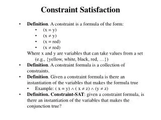
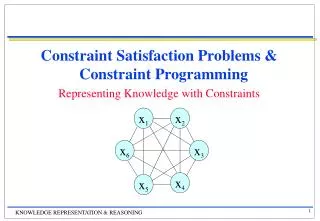
PROBLEM DEFINITION Problem / Input: A set of variables V {v1, v2, …, vn} Each variable has a domain: D1, D2, … Dk, for k≤n all variables may have the same domain A set of constraints C {c1, c2, … cm}, m ≤ nChoosearity In a constraint-graph, constraints are labels on arcs; typically binary constraints, binary graph, (arity=2)but multi-aried is feasible; arity=1 is ok too (restricted domain) Constraint ci connects a subset of variables’ (arity) for SIMULTANEOUS “allowed” values e.g., C = {(v1=blue, v2=green), (v1=green, v2=blue)} (C) Debasis Mitra
Example Constraint ci connects a subset of variables’ (arity) for “allowed” SIMULTANEOUS values V = {v1, v2, v3} D for all v’s = { red, blue, green, yellow} C = {{v1-v2, (red, green), (blue, green) – think of a table}, { v1-v3, (yellow, green), (green, yellow)} } Note: no constraint on v2-v3; inherently directed v1 {green, red}, {green, blue} {yellow, green} {green, yellow} v3 v2 CSP: is this input satisfiable? T/F Answer: False (try it) (C) Debasis Mitra
Example 2 V = {v1, v2, v3} D1= {1, 2, 3}, D2={1, 4}, D3={3, 5} // Disjunctive: chose any C = {v1 < v2, v2<v3} // Constraints are conjunctive: all must satisfy CSP: is this input satisfiable? Output: True A solution: (v1, v2, v3)=(1, 4, 5) All solutions? Exercise… v1 < < v3 v2 “Filtered” network note v3=3 is not feasible, does not appear in any solution (C) Debasis Mitra
CONSTRAINT GRAPH Typical: binary (we know about binary graph well) Graph structure may be exploited: Tree – easy to handle (why?) Multi-aried constraints = “Global constraints” e.g., “alldiff” = vars have same domains, & each must be unique Graph = Propositional Logic Constraint Logic Programming: goes beyond Prop-Logic Dual graph: Interchange nodes and arcs Dual representation may be valuable! Think Interior-Point algorithm for LP. (C) Debasis Mitra
CONSTRAINT EXAMPLES Map coloring: Book Ch 6 Slides 4-6 [DRAW ON BOARD] Cryptarithmatic Example: Book Ch 6 slide 9 Other list: Ch 6 Slide 10 (C) Debasis Mitra
GENERATE A SOLUTIONOR FAILURE Book Ch 6 Slides 11: Formulation as a search problem • Let's start with the straightforward, dumb approach, then fix it. • States are defined by the values assigned so far • Initial state: the empty assignment, {v1=null, v2=null, … } • Successor function: assign a value to an unassigned variable • that does not conflict with current assignment. • => fail if no legal assignments (constraints not satisfiable! CSP->False) • Goal test: the current assignment is complete • 1) This is the same for all CSPs! • 2) Every solution appears at depth d=n, for n variables • => use depth-first search • 3) Path is irrelevant, so, algorithm can also use complete-state formulation • 4) b=(n - l)*d at depth l, (l goes from 0 to d ), hence bn ~n!dn leaves!!!! (C) Debasis Mitra
GENERATE A SOLUTIONOR FAILURE Book Ch 6 Slides 12-26: Backtracking DFS Heurstics-based improvements Forward Checking (C) Debasis Mitra
CONSTRAINT REASONING/SEARCH ISSUES In terms of Logic: Inferencing 1. How do you answer the questions (T/F)? 2. Produce required output (one or more solutions)? 3. “Filter” the domains constraints (discard impossibilities), so that some values/constraint elements that will never take part in any solution are eliminated. Algorithms: Backtracking Forward Checking Constraint Propagation, at different “levels” (C) Debasis Mitra
CONSTRAINT REASONING / SEARCH ISSUES:Filtering / Propagation How to “filter” the domains (on nodes) and constraints (on arcs), so that, those values/constraint elements which will never take part in any solution are eliminated? Algorithms produce some type of “filtered” outputs! Or, Failure! Different levels of filtering defines different levels of CONSISTENCY (C) Debasis Mitra
CONSISTENCY TYPES • Simplest, Node consistency • Constraint of arity=1, Unary constraints • Domain is “constrained” within list of input constraints • Some values are explicitly prohibited, • e.g., in job-shop-scheduling: No class may start before 8 am; Grad classes may not start before 4pm • If a “solution” (e.g., a schedule) satisfies “Node consistency”, then, the solution is “Node consistent” • Or, “After” filtering each variable per Node constraints, the constraint network is “Node consistent” • A confusing issue is the input is x-consistent “before” or “after” filtering? (C) Debasis Mitra
ARC CONSISTENCY (AC) • Constraint of arity=2, Binary constraints Eliminate domain values that does not have any support on the other variable according to each constraint Example: v1 = {1, 2, 3}, v2={2,3,4}, v3=… Constraints: v1=v2, … Filter (AC) between v1-v2: v1={1, 2, 3}, v2={2, 3, 4}, … But then this may cause other variables to loose support --- (C) Debasis Mitra
ARC CONSISTENCY (AC) • Constraint of arity=2, Binary constraints Eliminate domain values that does not have any support on the other variable according to each constraint Example: v1 = {1, 2, 3}, v2={2,3,4}, v3={4, 5, 7} Constraints: v1=v2, v2=v3 Filter (AC) between v1-v2: v1={1, 2, 3}, v2={2, 3, 4}, v3={4, 5, 7} Therefore, CSP: F --- --- (C) Debasis Mitra
ARC CONSISTENCY (AC) • Constraint of arity=2, Binary constraints Eliminate domain values that does not have any support on the other variable according to constraint Example: v1 = {1, 2, 3}, v2={2,3,4}, v3={1,2,3}, … Constraints: v1=v2, v2<v3,… Filter (AC) between v1-v2: v1={1, 2, 3}, v2={2, 3, 4} Filter (AC) between v2-v3: v2={2, 3}, v3={1,2,3}, … and so on, until no more change in the graph (C) Debasis Mitra
ARC CONSISTENCY • Constraint of arity=2, Binary constraints Eliminate domain values that does not have any support on the other variable according to the constraints • Not as easy as it appears! • Domains are to be filtered, or reduced, or shrunk • Need to repeat again and again: • every value elimination needs to propagate • But how many times? • Easiest algorithm: Keep repeating until no more variable changes OR: a domain becomes null Inconsistent (CSP: F) Any variable value-set changes: check its neighbors use a Queue_of_arcs (AC-3) (C) Debasis Mitra
AC-3: ARC CONSISTENCY ALGORITHM • Book Ch 6 Slides 27-31 (C) Debasis Mitra
ARC CONSISTENCY • Easiest algorithm: Keep “filtering” per arc-constraints until no more variable changes, OR: a domain becomes null Inconsistent (CSP: F) (on a CSP=F, if you do not do the last step all domains will become ‘null’) • After filtering each variable per Arc constraints, the constraint network is “Arc consistent” (AC) • AC network ≡ every variable value will have a corresponding variable value at the other end of its constraints • Not same as “Satisfiability”: an Arc consistent network may not actually have any solution: 2-color on Australia AC has a sol, but not solution • Then, what good is AC? 1) It will be faster to find solution on an AC network! 2) But more importantly: may find inconsistency quickly P-time (C) Debasis Mitra
PATH CONSISTENCY • Really, Triangle Consistency • Constraints (≡allowed value pairs) are filtered such that each constraint will satisfy every triangle it participates in • A theorem proves, this is same as participating in any path it resides in • More filtering than AC • PC ≠ AC, strange! • PC-2 per Mackworth et al. is very similar to AC-3, with triangles instead of arcs Examples on AC, PC, etc.: http://cs.fit.edu/~dmitra/ArtInt/TextSlides/constraints-dechter-2 (C) Debasis Mitra
k-CONSISTENCY • k=1: node consistency • k=2: AC • k=3: PC • k-consistency = every (k-1)-nodes value-set has extension to k-th node • k>3: does not imply (k-1)-consistency • If a network is filtered such that it is k=1, … p-consistent, then, it is called Strongly-p consistent • Strongly k-consistent for k=n, for n nodes network Global consistent • Minimal Network: eachdomain value participates in a solution a backtrack free search may used to find a solution (but, finding a solution/Failure may be easier than min-net!) (C) Debasis Mitra
BOUND-CONSISTENCY • On Ordinal / Real domains • Constraints are over ranges, range = bound • Range gets filtered on bound propagation • “Simple” bounds = convex (single) ranges on each domain (& constraints) • => Bound propagation for convex bounds only, is P-class, • Global consistency (finding satisfiable value for each node by backtrack-free search) • Non-simple bounds on input (=multiple or non-convex ranges) => NP-complete B [10-20] A (C) Debasis Mitra
CONSISTENCY • Run a path-consistency algorithm on input constraint network P: • Does P change? • If “yes”: P was not 3-consistent • If “no”: P was 3-consistent • k-consistency, for k=1, 2 (Arc-cons.), 3 (Path-cons.), … • k-consistent network does not necessarily imply (k-1) • Weak k-consistent: only k-consistent network • Strong k-consistent: i-consistent for i=1, …k • Satisfiable: There exists a non-null solution. • k-sat: solution exists for every k-subgraph (may be k=1, 2, … n, for n var) • Weaker than consistency definition [WHY?] Counter-examples: http://cs.fit.edu/~dmitra/ArtInt/TextSlides/constraints-tsang-1 (C) Debasis Mitra
STRUCTURE OF NETWORK • Book Slides 32-36 • [slide 33 may be loaded -> mention Kadison-Singer] • Phase Transition: Book Slide 39 (C) Debasis Mitra
MORE ON CONSTRAINTS • Finding Solution(s): Backtracking • Different from inferencing/propagation • Assign value on nodes without violating constraints • Which var v to pick next? Which value of v to pick next? • Run-time depends on above • Branching factor: nd, n=|V|, d=|D| • And-Or tree: And on nodes (need all nodes values), Or on values (any value will do) • A node empty Fail, Each value must be tried before a node fails • Complexity = #nodes on search tree = nd*(n-1)d*(n-2)d*…=n!dn • # possible node-value assignments = dn , some of them are solutions • Think of 2n Boolean-SAT problem • Strategy, heuristics, pruning, … to improve search (C) Debasis Mitra
BACKTRACKING Var-ordering: • Min-remaining Values (MRV): choose var with fewest remaining values • Most-constrained var (MCN): maximum degree node • Fail-first strategy: better pruning • Of course, out of remaining unassigned nodes • A good tie-breaker after MRV Value-ordering: • Least constraining value: this value allows others to satisfy easily • Note: values are disjunctive, whereas constraints are conjunctive (MCN above) (C) Debasis Mitra
BACKTRACKING (BT) • Interleaving: • Backtrack search interleaved with constraint propagation • Forward Checking (FC): BT + AC • FC is redundant if AC is run first, before running BT • MAC (maintaining AC): BT + AC only on subgraph for the current Xi, and all unassigned Xj’s (C) Debasis Mitra
BACKTRACKING: Look Back(EXCLUDE THIS SLIDE) • Ordinarily backtrack to previous var on search tree • Look-back strategies: Jump back to more relevant node • More pruning • Backjumping (BJ): • Conflict-directed backjumping (CBJ) • Who caused the conflict that lead to failure of current node? • Learning-based backjumping (LBJ) • Keep track of “no-good” value assignments: actually implied constraint • But only maximal “no-good” is useful: that cannot be extended in the network • Use no-goods as a new constraint to filter domains (or use any other ways!) (C) Debasis Mitra
LOCAL SEARCH: CONSTRAINTS • Not progressing variable to variable: state-based • Min-conflict: • n-queens: Choose a random var, flip value that conflicts most • Good when solutions are densely distributed in search space • Simulated Annealing: Need a heuristic of “goodness” • Genetic Algorithm: Need a good representation for splitting • WalkSat: http://cs.fit.edu/~dmitra/ArtInt/TextSlides/constraints-dechter-1 • Constraint dynamic weighting: • Assign weight to constraints per its violation history • Choose var-value pair that minimizes total violated constraint weights http://cs.fit.edu/~dmitrTextSlides/constraints-dechter-1 (C) Debasis Mitra
MORE ON CONSTAINTS: GRAPH STRUCTURE • Tree structure: • Topological sort nodes, then run directed AC (DAC) • DAC: ordered nodes filter forward/downward • Guaranteed linear=bt-free search to assign value • P-class problem: polynomial-time satisfiability check • (more or less what happens for 2-SAT problem!) • Almost tree: • Remove a node and it becomes tree (Australia-coloring, SA is such a node) • Such nodes are called “cycle cutset” • Needs to backtrack only on cycle-cutset • apply heuristics/strategies on cutset to make algo even faster • Group nodes together to super-node and convert graph to a tree • Each group’s solutions become domain for the supernode (Fig 6.13) • Sort of polynomial ~ dc for fixed tree size c, instead of ~dn • Can we use strongly connected components? (C) Debasis Mitra
MORE ON CONSTAINTS • Value Symmetry: • Solutions are agnostic to the names of colors: categorical data • Permutations of color-names (n!) of a solution are really same solution • Search space may be reduced by introducing symmetry-breaking constraints • Note how symmetry may be used to exclude 15-puzzle’s unsolvable cases • We are just scratching the surface of symmetry in data! • Think of “Big Data” (C) Debasis Mitra
MORE ON CONSTAINTS • Sudoku problem as exercise? • 81 variables, partial-solution, 27 all-diff constraints • AC-3 gets close for most problems • PC-2 gets harder ones • Many inferencing strategies exist (C) Debasis Mitra
MORE ON CONSTAINTS(EXCLUDE THIS SLIDE) • Tractable sub-problems • Full problem is NP-hard: we looked for strategies, heuristics • Look for subproblems where satisfiability may be P: Tree structure • Constraint Logic Programming • Multi-aried • Higher-order logic: variable bindings • Prolog to express constraint network: • Variables with data as domain constraints + Rules as constraints = database+relations • Datalog, “Answer Set Programming” • Learning Constraints from Data? • Relational learning from database: find dependencies between attributes (C) Debasis Mitra
5 Algorithms: AC-3, PC-2, DPLL, Walk-SAT, CBJ (EXCLUDE SCRATCHED ONES) (C) Debasis Mitra
AC-3 function AC3(R) Input: a binary network R = (V, D, C) Output: an equivalent path-consistent network R’ or False 0 R’ = R // make a copy 1 a queue Q of arcs initialized with all arcs in R, Q {(i,j) | 1≤i<j ≤ n} 2 while Q is not empty do 3 select and remove an arc (i, k) from Q 4 Temp_Di = values in Di that has corresponding value in Dk following constraint Cik 5 if Temp_Di== Null then return False 6 if Temp_Di ≠ Di then 7 replace Di with Temp_ Di in R’ 8 Push-in(Q, {arcs (p, i), for all p ≠ i, i.e. all arcs in which i participates} end while 9 return R’ (C) Debasis Mitra
PC-2 function PC-2(R) Input: a binary network R = (V, D, C) Output: an equivalent path-consistent network R’ or False 0 R’ = R // make a copy 1 a queue Q of triangles initialized with all triangle in R, Q {(i,j,k) | 1 ≤ i<j ≤ n, 1 ≤ k ≤ n, k ≠i, k ≠ j} 2 while Q is not empty do 3 select and remove a 3-tuple (i, j, k) from Q 4 Temp_Cij = \project on ij (Cik \join Dk \join Cjk) // \project and \join explained on next slide 5 Cij’ Cij \intersect Temp_Cij 6 if Cij’ = = Null return False 7 if Cij’ has changed from Cij then 8 replace Cij with Cij’ in R’ 9 Push-in(Q, {triangles (p, j, i), for all p ≠ i, and p ≠ j, i.e. all triangles in which ij participates} end while 10 return R’ (C) Debasis Mitra
For those who may not have been exposed to Relational Algebra: (Cik \join Dk \join Cjk) means creating new constraints Cikj such that each triple of value has corresponding support in Cij, Dk, and Cjk Example: Cij = (<r,3>, <b,5>), Dk = (3, 6), Cjk = (<3,g>,<5,b>) Then, Cijk by above joins will be = (<r,3,g>) \projectij shrinks the constraint to variables ij pair, thus from above Cijk, \projectij Cijk = (<r,g>) (C) Debasis Mitra
Algorithm DPLL (for Boolean satisfiability or SAT-problem) Input: A set of clauses Φ. Output: A Truth Value. function DPLL(Φ) if Φ is a consistent set of literals then return true; if Φ contains an empty clause then return false; for every unit clause l in Φ// unit clause, clause with one literal Φ ← unit-propagate(l, Φ);// make the literal true in all clauses for every literal l that occurs pure in Φ// either + or – in all clauses Φ ← pure-literal-assign(l, Φ);// assign its value to make it T l ← choose-literal(Φ); return DPLL(Φ ∧ l) or DPLL(Φ ∧ not(l)); // Binary tree search Source: Wiki (C) Debasis Mitra
GSAT and Walksat algorithms work on formulae in Boolean logic that are in, or have been converted into, conjunctive normal form. They start by assigning a random value to each variable in the formula. If the assignment satisfies all clauses, the algorithm terminates, returning the assignment. Otherwise, a variable is flipped and the above is then repeated until all the clauses are satisfied. WalkSAT and GSAT differ in the methods used to select which variable to flip. GSAT makes the change which minimizes the number of unsatisfied clauses in the new assignment, or with some probability picks a variable at random, somewhat like simulated annealing with fixed T. WalkSAT first picks a clause which is unsatisfied by the current assignment, then flips a variable within that clause. The clause is picked at random among unsatisfied clauses. The variable is picked that will result in the fewest previously satisfied clauses becoming unsatisfied, with some probability of picking one of the variables at random. When picking at random, WalkSAT is guaranteed at least a chance of one out of the number of variables in the clause of fixing a currently incorrect assignment. When picking a guessed “to be optimal” variable, WalkSAT has to do less calculation than GSAT because it is considering fewer possibilities. The algorithm may restart with a new random assignment if no solution has been found for too long, as a way of getting out of local minima of numbers of unsatisfied clauses. Source: Wiki (C) Debasis Mitra