Download
1 / 63
640 likes | 923 Vues
Electronic Absorption Spectroscopy of Organic Compounds. W. R. Murphy, Jr. Department of Chemistry and Biochemistry Seton Hall University. Course Topics. UV absorption spectroscopy Basic absorption theory Experimental concerns Chromophores Spectral interpretation Chiroptic Spectroscopy

E N D
Electronic Absorption Spectroscopy of Organic Compounds W. R. Murphy, Jr. Department of Chemistry and Biochemistry Seton Hall University
Course Topics • UV absorption spectroscopy • Basic absorption theory • Experimental concerns • Chromophores • Spectral interpretation • Chiroptic Spectroscopy • ORD, CD • Effects of inorganic ions (as time permits)
Electric and magnetic field components of plane polarized light • Light travels in z-direction • Electric and magnetic fields travel at 90° to each other at speed of light in particular medium • c (= 3 × 1010 cm s-1) in a vacuum
Wavelength and Energy Units • Wavelength • 1 cm = 108Å = 107 nm = 104 =107 m (millimicrons) • N.B. 1 nm = 1 m (old unit) • Energy • 1 cm-1 = 2.858 cal mol-1 of particles = 1.986 1016 erg molecule-1= 1.24 10-4 eV molecule-1 • E (kcal mol-1) (Å) = 2.858 105 • E(kJ mol-1) = 1.19 105/(nm)297 nm = 400 kJ
Absorption Spectroscopy • Provide information about presence and absence of unsaturated functional groups • Useful adjunct to IR • Needed for chiroptic techniques • Determination of concentration, especially in chromatography • For structure proof, usually not critical data, but essential for further studies • NMR, MS not good for purity
Importance of UV data • Particularly useful for • Polyenes with or without heteroatoms • Benzenoid and nonbenzenoid aromatics • Molecules with heteroatoms containing n electrons • Chiroptic tool to investigate optically pure molecules with chromophores • Practically, UV absorption is measured after NMR and MS analysis
UV and Visible Spectroscopy • Vacuum UV or soft X-rays • 100 - 200 nm • Quartz, O2 and CO2 absorb strongly in this region • N2 purge good down to 180 nm • Quartz region • 200 – 350 nm • Source is D2 lamp • Visible region • 350 – 800 nm • Source is tungsten lamp
All organic compounds absorb UV-light • C-C and C-H bonds; isolated functional groups like C=C absorb in vacuum UV; therefore not readily accessible • Important chromophores are R2C=O, -O(R)C=O, -NH(R)C=O and polyunsaturated compounds
Spectral measurement • usually dissolve 1 mg in up to 100 mL of solvent for samples of 100-200 D molecular weight • data usually presented as A vs (nm) • for publication, y axis is usually transformed to or log10 to make spectrum independent of sample concentration
Preparation of samples • Concentration must be such that the absorbance lies between 0.2 and 0.7 for maximum accuracy • Conjugated dienes have 8,000-20,000, so c 4 10-5 M • n* of a carbonyl have 10-100, so c 10-2 M • Successive dilutions of more concentrated samples necessary to locate all possible transitions
Solvent choices • Important features to consider are solubility of sample and UV cutoff of solvent • Filtration to remove particulates is useful to reduce scattered light • Solvent purity is very important
Chromophores • Structures within the molecule that contain the electrons being moved by the photon of light • Only those absorbing above 200 nm are useful • n* in ketones at ca 300 nm is only isolated chromophore of interest • all other chromophores are conjugated systems of some sort
Molecular orbitals for common transitions • Molecular orbital diagram for 2-butenal • Shows n * on right • Shows * on left • Both peaks are broad due to multiple vibrational sublevels in ground and excited states
Beer’s Law • Io = Intensity of incident light • I = Intensity of transmitted light • = molar extinction coefficient • l = path length of cell • c = concentration of sample
Transition Energies • Electronic transitions are quantized, so sharp bands are expected • In reality, absorption lines are broadened into bands due to other types of transitions occurring in the same molecules • For electronic transitions, this means vibrational transitions and coupling to solvent
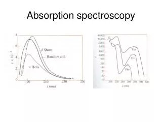
Vibrational fine structure • Rigid molecules such as benzene and fused benzene ring structures often display vibrational fine structure • Example is benzene in heptane • Usually only observed in gas phase, but rigid molecules do display this
Intensities of transitions • Strictly speaking, one should work with integrated band intensities • However, overlap of bands prevents clean isolation of transitions (hence the popularity of fluorescence in photophysical studies) • Therefore, intensities are used
Selection Rules • After resonance condition is met, the electromagnetic radiation must be able to electrical work on the molecule • For this to happen, transition in the molecule must be accom-panied by a change in the electrical center of the molecule • Selection rules address the requirements for transitions between states in molecules • Selection rules are derived from the evaluation of the properties of the transition moment integral (beyond scope of this course
Selection Rule Terminology • Transitions that are possible according to the rules are termed “allowed” • Such transitions are correspond-ingly intense • Transitions that are not possible are termed “forbidden” and are weak • Transitions may be “allowed” by some rules and “forbidden” by others
Common Selection Rules • Spin-forbidden transitions • Transitions involving a change in the spin state of the molecule are forbidden • Strongly obeyed • Relaxed by effects that make spin a poor quantum number (heavy atoms) • Symmetry-forbidden transitions • Transitions between states of the same parity are forbidden • Particularly important for centro-symmetric molecules (ethene) • Relaxed by coupling of electronic transitions to vibrational transitions (vibronic coupling)
Intensities • P is the transition probability; ranges from 0 to 1 • a is the target area of the absorbing system (the chromophore) • chromophores are typically 10 Å long, so a transition of P = 1 will have an of 105
Intensities, con’t. • this intensity is actually observed, and has been exceeded by very long chromophoric systems • Generally, fully allowed systems have > 10,000 and those with low transition probabilities will have < 1000 • Generally, the longer the chromophore, the longer wavelength is the absorption maximum and the more intense the absorption
Intensities - Important forbidden transitions • n* • near 300 nm in ketones • ca 10 - 100 • In benzene and aromatics • band around 260 nm and equivalent in more complex systems • > 100 • Prediction of intensities is a very deep subject, covered in Physical Methods next year
Fundamentals of spectral interpretation • Examining orbital diagrams for simple conjugated systems is helpful (lots of good programs available to do these calculations) • Wavelength and intensity of bands are both useful for assignments
Solvent effects • Franck-Condon Principle • nuclei are stationary during electronic transitions • Electrons of solvent can move in concert with electrons involved in transition • Since most transitions result in an excited state that is more polar than the ground state, there is a red shift (10 - 20 nm) upon increasing solvent polarity (hexane to ethanol)
Solvent effects Hydrocarbons water • * • Weak bathochromic or red shift • n* • Hypsochromic or blue shift (strongly affected by hydrogen bonding solvents) Solvent effects due to stabilization or destabilization of ground or excited states, changing the energy gap
Solvent effects, con’t • n* in ketones is the exception • there is a blue shift • this is due to diminished ability of solvent to hydrogen bond to lone pairs on oxygen • example - acetone • in hexane, max = 279 nm ( = 15) • in water, max = 264.5 nm
Band assignments: n* • < 2000 • Strong blue shift observed in high dielectric or hydrogen-bonding solvents • n* often disappear in acidic media due to protonation of n electrons • Blue shifts occur upon attachment of an electron-donating group • Absorption band corresponding to the n* is missing in the hydrocarbon analog (consider H2C=O vs H2C=CH2 • Usually, but not always, n* is the lowest energy singlet transition • * transitions are considerably more intense
Searching for chromophores • No easy way to identify a chromophore • too many factors affect spectrum • range of structures is too great • Use other techniques to help • IR - good for functional groups • NMR - best for C-H
Identifying chromophores • complexity of spectrum • compounds with only one (or a few) bands below 300 nm probably contains only two or three conjugated units • extent to which it encroaches on visible region • absorption stretching into the visible region shows presence of a long or polycyclic aromatic chromophore
Identifying chromophores • Intensity of bands - particularly the principle maximum and longest wavelength maximum • Simple conjugated chromophores such as dienes and unsaturated ketones have values from 10,000 to 20,000 • Longer conjugated systems have principle maxima with correspondingly longer max and larger
Identifying chromophores • Low intensity bands in the 270 - 350 nm (with ca 10 - 100) are result of ketones • Absorption bands with 1000 - 10,000 almost always show the presence of aromatic systems • Substituted aromatics also show strong bands with > 10,000, but bands with < 10,000 are also present
Next steps in spectral interpretation • Look for model systems • Many have been investigated and tabulated, so hit the literature • Major references • Organic Electronic Spectral Data, Wiley, New York, Vol 1-21 (1960-85) • Sadtler Handbook of Ultraviolet Spectra, Heyden, London
Substituted acyclic dienes • max shifts • Presence of substituents • Length of conjugation