Get Folder
Learn about the intricate interplay of basic elements and interactions shaping complex, random behaviors in economics and physics. Discover the historical figures and notable books in this field and delve into the statistical physics that underpins financial markets. Uncover the parallels between statistical physics and financial markets, how agents interact in trading decisions, and the social imitation theory influencing market dynamics. Delve into topics like cooperative phenomena and non-linear complexity, understanding opinion changes and trader dynamics. Get insights into stock dynamics, risk management, and empirical stock market trends, exploring the scientific method in economics and the intricacies of financial market complexities.

Get Folder
E N D
Presentation Transcript
Get Folder • Network Neighbourhood • Tcd.ie • Ntserver-usr • Get • richmond
Econophysics Physics and Finance (IOP UK) Socio-physics (GPS) Molecules > people Physics World October 2003 http://www.helbing.org/ Complexity Arises from interaction Disorder & order Cooperation & competition Stochastic Processes Random movements Statistical Physics cooperative phenomena Describes complex, random behaviour in terms of basic elements and interactions
Physics and Finance-history • Bankers • Newton • Gauss • Gamblers • Pascal, Bernoulli • Actuaries • Halley • Speculators, investors • Bachelier • Black Scholes >Nobel prize for economics
Books – Econophysics • Statistical Mechanics of Financial Markets • J Voit Springer • Patterns of Speculation; A study in Observational Econophysics • BM Roehner Cambridge • Introduction to Econophysics • HE Stanley and R Mantegna Cambridge • Theory of Financial Risk: From Statistical Physics to Risk Management • JP Bouchaud & M Potters Cambridge • Financial Market Complexity • Johnson, Jefferies & Minh Hui Oxford
Books – Financial math • Options, Futures & Other Derivatives • JC Hull • Mainly concerned with solution of Black Scholes equation • Applied math (HPC, DCU, UCD)
Books – Statistical Physics • Stochastic Processes • Quantum Field Theory (Chapter 3) Zimm Justin • Langevin equations • Fokker Planck equations • Chapman Kolmogorov Schmulochowski • Weiner processes; diffusion • Gaussian & Levy distributions • Random Walks & Transport • Statistical Dynamics, chapter 12, R Balescu • Topics also discussed in Voit
Read the business press • Financial Times • Investors Chronicle • General Business pages • Fundamental & technical analysis • Web sites • http://www.digitallook.com/ • http://www.fool.co.uk/
Perhaps you want to become an actuary. Or perhaps you want to learn about investing? Motivation What happened next?
Questions • Can we earn money during both upward and downward moves? • Speculators • What statistical laws do changes obey? What is frequency, smoothness of jumps? • Investors & physicists/mathematicians • What is risk associated with investment? • What factors determine moves in a market? • Economists, politicians • Can price changes (booms or crashes) be predicted? • Almost everyone….but tough problem!
Why physics? • Statistical physics • Describes complex behaviour in terms of basic elements and interaction laws • Complexity • Arises from interaction • Disorder & order • Cooperation & competition
Financial Markets • Elements = agents (investors) • Interaction laws = forces governing investment decisions • (buy sell do nothing) • Trading is increasingly automated using computers
Social Imitation Theory of Social Imitation Callen & Shapiro Physics Today July 1974Profiting from Chaos Tonis Vaga McGraw Hill 1994 buy Hold Sell
Are there parallels with statistical physics? E.g. The Ising model of a magnet Focus on spin I: Sees local force field, Yi, due to other spins {sj} plus external field, h I h
Mean Field theory • Gibbsian statistical mechanics
Jij=J>0 Total alignment (Ferromagnet) • Look for solutions <σi>= σ σ = tanh[(J σ + h)/kT] +1 -h/J σ*>0 y= tanh[(J σ+h)/kT] y= σ -1
Orientation as function of h y= tanh[(J σ+h)/kT] ~sgn [J σ+h] +1 Increasing h -1
Spontaneous orientation (h=0) below T=Tc T<Tc +1 T>Tc σ* Increasing T
Social imitation • Herding – large number of agents coordinate their action • Direct influence between traders through exchange of information • Feedback of price changes onto themselves
Opinion changesK Dahmen and J P Sethna Phys Rev B53 1996 14872J-P Bouchaud Quantitative Finance 1 2001 105 • magnets si trader’s position φi (+ -?) • field h time dependent random a priori opinion hi(t) • h>0 – propensity to buy • h<0 – propensity to sell • J – connectivity matrix
Confidence? • hi is random variable • <hi>=h(t); <[hi-h(t)]2>=Δ2 • h(t) represents confidence • Economy strong: h(t)>0 • expect recession: h(t)<0 • Leads to non zero average for pessimism or optimism
Need mechanism for changing mind • Need a dynamics • Eg G Iori
Topics • Basic concepts of stocks and investors • Stochastic dynamics • Langevin equations; Fokker Planck equations; Chapman, Kolmogorov, Schmulochowski; Weiner processes; diffusion • Bachelier’s model of stock price dynamics • Options • Risk • Empirical and ‘stylised’ facts about stock data • Non Gaussian • Levy distributions • The Minority Game • or how economists discovered the scientific method! • Some simple agent models • Booms and crashes • Stock portfolios • Correlations; taxonomy
Basic material • What is a stock? • Fundamentals; prices and value; • Nature of stock data • Price, returns & volatility • Empirical indicators used by ‘professionals’ • How do investors behave?
characterises occurrence of random variable, X For all values of x: p(x) is positive p(x) is normalised, ie: -/0 p(x)dx =1 p(x)x is probability that x < X < x+x a b p(x)dx is probability that x lies between a and b Probability distribution density functions p(x)
Cumulative probability function C(x) = Probability that x<X = - x P(x)dx = P<(x) P>(x) = 1- P<(x) C() = 1; C(-) = 0
Average and expected values For string of values x1, x2…xN average or expected value of any function f(x) is In statistics & economics literature, often find E[ ] instead of
Moments and the ‘volatility’ m n < xn > = p(x) xn dx Mean: m 1 = m Standard deviation, Root mean square (RMS) variance or ‘volatility’: 2 = < (x-m)2 > = p(x) (x-m)2dx = m2 – m 2 NB For mn and hence to be meaningful, integrals have to converge and p(x) must decrease sufficiently rapidly for large values of x.
Gaussian (Normal) distributions PG(x) ≡ (1/(2π)½σ) exp(-(x-m)2/22) All moments exist For symmetric distribution m=0; m2n+1= 0 and m2n = (2n-1)(2n-3)…. 2n Note for Gaussian: m4=34 =3m22 m4is ‘kurtosis’
Some other Distributions Log normal PLN(x) ≡ (1/(2π)½ xσ) exp(-log2(x/x0)/22) mn = x0nexp(n22/2) Cauchy PC (x) ≡ /{1/(2 +x2)} Power law tail (Variance diverges)
Levy distributions NB Bouchaud uses instead of Curves that have narrower peaks and fatter tails than Gaussians are said to exhibit ‘Leptokurtosis’
Simple example • Suppose orders arrive sequentially at random with mean waiting time of 3 minutes and standard deviation of 2 minutes. Consider the waiting time for 100 orders to arrive. What is the approximate probability that this will be greater than 400 minutes? • Assume events are independent. • For large number of events, use central limit theorem to obtain m and . • Thus • Mean waiting time, m, for 100 events is ~ 100*3 = 300 minutes • Average standard deviation for 100 events is ~ 2/100 = 0.2 minutes • Model distribution by Gaussian, p(x) = 1/[(2)½] exp(-[x-m]2/22) • Answer required is • P(x>400) = 400 dx p(x) ~ 400 dx 1/((2)½) exp(-x2/22) • = 1/()½z dy exp(-y2) • where z = 400/0.04*2 ~ 7*10+3 • =1/2{ Erfc (7.103)} = ½ {1 – Erf (7.103)} • Information given: 2/ * z dy exp(-y2) = 1-Erf (x) • and tables of functions containing values for Erf(x) and or Erfc(x)


