
Chapter 4
Chapter 4. The Root locus Method. Chapter 4 Root locus Method. 4.1 Introduction 4.2 The concepts of the root-locus 4.3 The root locus sketching(conventional root-locus) 4.4 The parameter root-locus and the zero-degree root-locus

Chapter 4
E N D
Presentation Transcript
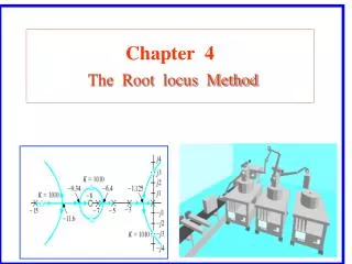
Chapter 4 The Root locus Method
Chapter 4 Root locus Method 4.1 Introduction 4.2 The concepts of the root-locus 4.3 The root locus sketching(conventional root-locus) 4.4 The parameter root-locus and the zero-degree root-locus 4.5 The Root loci of the system with the time-delay 4.6 The control system analysis and design utilizing the root- loci method
4.1 Introduction For investigating the performance of a system, we have to solve the output response of the system. But there are two defects when we do this: (1) It is a difficult thing to solve the output responseof a system – especially for a higher order system. (2) We can’t easily investigate the changes of a system’s performancefrom the time-domain solution of the system’s output response when one or two parameters of the system varies in a given range, or, when one or more devices are added to the system to improve the system’s. We can utilize the Root-locus technique to make up for the defects above. Root-locusis a graphical technique base on f the poles and zeros of the open-loop transfer function for determining the poles of the closed-loop transfer function of a system. Utilizing Root-locus technique, We can easily investigatethe performance changewhen one or two parameters of the system varies in a given range:
(basic conception of the root-locus). (plotting) (analysis of the root locus) 4.1 Introduction • when some parameter of the system varies in a given range; • when some device is added to the system. • The root-locus technique can be conveniently used for designing and analyzing the control systems. History: Root-locus method was conceived by Evans in 1948. Root-locus method and Frequency Response method, which was conceived by Nyquist in 1938 and Bode in 1945, make up of the cores of the classical control theory for designing and analyzing control systems. We discuss the root-locus according to following order: 1). what is Root-locus? 2). How the root-locus plot of a system is sketched? 3). How the performance information is analyzed from the root locus of a system.
R(s) C(s) Fig.4.1 4. 2 The Root locus concept 4.2.1 What is the root locus of a system? Example 4.1:for thesystem shown in Fig.4.1: The open-loop transfer function: The characteristic equation: The roots of the characteristic equation, or the poles of the closed loop transfer function of the system:
Discuss the s1and s2 varying with k from 0 to ∞ in S-plane According to above discussion: we can sketch the locus of the roots varying with k from 0 to +∞ on the S-plane :
Fig.4.2 The root locus of the systemshown inFig.4.2 Fig. 4.2 The root loci of Example 4.1
Definition of Root locus: The root loci is the path of the roots of the characteristic equation, or the poles of the system’s closed-loop transfer function, traced out in the s-plane as a system parameter is changed. 4.2.2 What information can be got from the root-loci of the system? From Fig.4.2 we may obtain following information: 1) when k changes in the range 0 ~ +∞, the system is always stable, because the loci of the closed-loop poles are always in the left-half of the s-plane
4.3 Root loci sketching 4.3.1 Two Basic Criterion K1: the root-locus gain. 2. Two Basic criterion
4.3.2 The steps of the rapid sketching of the root locus The rapid sketching procedureof the root locusshown as follow: Basic approach:The complete root loci can be constructed point-by-point finding all points in the s-plane that satisfy the angle criterions. Demonstrate:
Step 4: determine the number of separate loci (root-locus branches) (1) The root-locus branches = n ( the number of the open-loop poles) Step 5:the root loci must be symmetrical with respect the horizontal real axis because the complex roots must appear as pairs of complex conjugate roots.
s s Demonstrate: Fig.4.4 Diagrammatizing 2 Fig.4.3 Diagrammatizing 1
Im Im Im Im Im Im Re Re Re Re Re Re Only in terms of above six steps we can rapidly sketch the root-loci of a control system. Sketch the root-loci for the following open-loop transfer functions: Example 4.2
Demonstratingθz is similar toθp . Example 4.3 The open-loop transfer function of a certain system is: Sketch the root locus of the system
Im Re Using the step 10 we have the solution Using the step 1 we have the characteristic equation: Using the step 2-6 we have: Using the step 9 we have the breakaway point: s1is thebreakaway point . Using the step 9 we have the asymptote: The root locus for example 4.3 The root locus shown in Fig. for example 4.3
4.4 Parameter Root Locus Conventional root locus Parameter Root Locus Parameter root locus --- the variable parameter of the control systems is another parameter besides K1 . We illustrate the parameter root locus and it’s sketching approaches by following example:
Im Re The procedure of sketching root locus is shown as following:
Im Re
Im Re
LoopⅠ Loop Ⅱ 4.4.2 The root-locus used for the multi-loop feedback system The root-locus also can be used for the multi-loop feedback systems. For example :
For these systems, the characteristic equations like as: 4.4.3 “Zero degree” root locus For example, sketch the root loci of the system with the open loop transfer function: Analysis:
,the sketching steps of If we substitute for the conventional root locus are also suitable to the“zero degree” root locus(only related to the step 6,7and10). So we have the “zero degree” root locus procedure: Example 4.5 Sketch the root loci of the system with the open loop transfer function: Solution This is a zero degree question.
If we consider K1 varying from 0→-∞ simultaneously, the root loci shown in Fig. Example 4.5 are named the “complete root loci”. Using the root loci procedures We can sketch the root loci shown in Fig. Example 4.5(red curves). Fig. Example 4.5
For the system with time delay The magnitude criterion: The angle criterion: Characteristic equation: We have: 4.5 Root loci of the system with time delay
The magnitude criterion: The angle criterion:
The magnitude criterion: The angle criterion:
Dominant root-locus 4.5 Root loci of the system with time delay
4.6 The control system analysis and design utilizing the root- loci method 4.6.1The effects on the system’s performance adding the open zeros or open poles 1. adding a open zero in the left s-plane For example Generally, adding a open zero in the left s-plane will lead the root loci to be bended to the left. And the more closer to the imaginary axis the open zero is, the more prominent the effect on the system’sperformance is.
4.6 The control system analysis and design utilizing the root- loci method 2. adding a open pole in the left s-plane For example Generally, adding a open pole in the left s-plane will lead the root loci to be bended to the right. And the more closer to the imaginary axis the open pole is, the more prominent the effect on the system’sperformance is.
4.6 The control system analysis and design utilizing the root- loci method 4.6.2the system’s performance analysis by root-loci method 1. We can get the information of the system’s stability in terms of that whether the root loci always are in the left-hand s-plane with the system’s parameter varying. 2. We can get some information of the system’s steady-state error in terms of the number of the open-loop poles at the origin of the s-plane. 3. We can get some information of the system’s transient performance in terms of the tendencies of the root loci with the system’s parameter varying, such as: • The root loci in the left-hand s-plane move to far from the imaginary axis with the system’s parameter varying, the system’s response is more rapid and the system is more stable, vice versa.
A unity feed back control system, the open-loop Transfer function is: 4.6 The control system analysis and design utilizing the root- loci method • The root loci in the left-hand of the s-plane move to far from the real axis with the system’s parameter varying, the oscillation of the system’s response is more acute and the percent overshoot is more bigger, vice versa. • We can approximately simplify a nth-order system to a second-order or a first-order system and make a quantitative analysis utilizing the dominant poles. Exercise p424 DP7.2; DP7.4 and Exercise 1. Polt the root locus of the system for K1=0~+∞。 2. Determine the transfer function of the controller of the system and K1 to make the steady-state error ess=0 for the unit ramp input and the percent overshoot σp%≤16.5% for the unit step input using the root-locus method.
2. make and 4.6 The control system analysis and design utilizing the root- loci method solution 1. the root locus of the system for K1=0~+∞ shown in Fig 4.6.3。 Can not fulfill the steady-state error requirement We have the open-loop transfer function of the system:


